International Journal of
Geo-Information Article
An Automatic Road Network Construction Method Using Massive GPS Trajectory Data Yongchuan Zhang 1,2, *, Jiping Liu 1,2 , Xinlin Qian 2 , Agen Qiu 1,2 and Fuhao Zhang 2 1 2
*
School of Resource and Environmental Sciences, Wuhan University, Wuhan 430079, China;
[email protected] (J.L.);
[email protected] (A.Q.) Chinese Academy of Surveying and Mapping, Beijing 100830, China;
[email protected] (X.Q.);
[email protected] (F.Z.) Correspondence:
[email protected] or
[email protected]; Tel.: +86-158-0134-0467
Received: 11 October 2017; Accepted: 1 December 2017; Published: 7 December 2017
Abstract: Automatically acquiring comprehensive, accurate, and real-time mapping information and translating this information into digital maps are challenging problems. Traditional methods are time consuming and costly because they require expensive field surveying and labor-intensive post-processing. Recently, the ubiquitous use of positioning technology in vehicles and other devices has produced massive amounts of trajectory data, which provide new opportunities for digital map production and updating. This paper presents an automatic method for producing road networks from raw vehicle global positioning system (GPS) trajectory data. First, raw GPS positioning data are processed to remove noise using a newly proposed algorithm employing flexible spatial, temporal, and logical constraint rules. Then, a new road network construction algorithm is used to incrementally merge trajectories into a directed graph representing a digital map. Furthermore, the average road traffic volume and speed are calculated and assigned to corresponding road segments. To evaluate the performance of the method, an experiment was conducted using 5.76 million trajectory data points from 200 taxis. The result was qualitatively compared with OpenStreetMap and quantitatively compared with two existing methods based on the F-score. The findings show that our method can automatically generate a road network representing a digital map. Keywords: digital map; road network construction; GPS trajectory; cartography
1. Introduction In the era of big data, people have increasing demands for comprehensive, accurate, and real-time navigational information, and the road network is the most important. For example, route planning, logistics, emergency rescue, and location-based services (LBSs) depend heavily on it. On the other hand, with the expansion of cities, new roads are being built, existing roads are being renovated from time to time, and traffic rules are being constantly updated, which lead to constantly changing road information (including the road network and traffic rules). Because the traditional acquiring and updating method of digital maps takes a great deal of human and material resources and the update cycle is long, changes are often not updated in a timely manner. For large cities such as Beijing and Shanghai, more than 40% of the map content should be updated every year; however, the traditional mapping method requires at least six months to update a map. Meanwhile, real-time traffic information has become an important part of navigational information. In this context, automatically obtaining highly accurate and near real-time road network information has become an important issue that needs to be solved urgently. An increasing number of public vehicles such as taxis, buses, and other public service vehicles are being equipped with global positioning system (GPS) devices. These vehicles produce considerable amounts of trajectory data. These trajectory data contain abundant information about the roads on ISPRS Int. J. Geo-Inf. 2017, 6, 400; doi:10.3390/ijgi6120400
www.mdpi.com/journal/ijgi
ISPRS Int. J. Geo-Inf. 2017, 6, 400
2 of 15
which those vehicles have traveled, and the information is recorded in real time, providing a new opportunity to collect and update road network information. However, automatically constructing a digital map in near real-time is a considerable challenge. First, it is difficult to determine whether several similar trajectories belong to the same road due to positioning errors. Second, the GPS positioning noise, vehicle speed, long position sampling cycle, and variable travel direction of vehicles make it difficult to separate and eliminate noise data. Third, the diversity and complexity of roads and urban infrastructures make it difficult to determine whether a position belongs to a particular road. Because of the above challenges, the production of digital maps requires manual editing in practice. For example, the creation of OpenStreetMap requires considerable manual editing. In this paper, we focus on automatically constructing a road network using GPS positioning data generated by taxis. The remainder of this paper is organized as follows. In Section 2, related studies are briefly reviewed. In Section 3, the problem of digital map construction from vehicle trajectory data and the details of our method are described. An experiment is carried out to validate the performance of our method in Section 4. Section 5 presents the conclusions from this work and suggested future work as a result of this paper. 2. Literature Review There are many road network information collection and updating methods, which can be divided into roughly three categories: (1) A specialized vehicle roaming road network [1] in which field operators drive specialized vehicles equipped with mapping devices and gather detailed road information, especially regarding the road network and related traffic regulations and points of interest (POIs). This method is professional and can be used to collect abundant information but is of low efficiency and requires a large investment. (2) Remote sensing image extraction [2,3], which first obtains the latest high-resolution remote sensing images or aerial photographs of the target area. Then, the initial information is extracted from these images and a field survey is conducted to collect other attribute information. This method is simple and fast, but newly updated road information cannot be collected economically or effectively because the images are expensive and the satellite revisit period is limited. (3) Volunteered geographic information (VGI) data extraction [4] in which volunteers such as students, navigational enthusiasts, and map lovers use their local advantages to gather the latest road information and provide it to the map producer. Then, the map producer can organize field survey workers to reconfirm and update the information. Often, up-to-date and detailed road information can be collected using this method but the quality of the updated data depends on the volunteers’ skills and the accuracy of the trajectory data; in addition, substantial post-processing must be performed to make the information useful. These methods are not exclusive; they are usually combined to obtain more comprehensive information. In certain commercial map companies such as AutoNavi and Google, the collection and updating of information for digital map construction are based mainly on data collected by specialized vehicles that roam the road network and remote sensing image extraction. Along with the development of mobile positioning technology, many scholars have recently explored the extraction and updating of road information from trajectory data [5–7]. These trajectory data are mainly of two types: positioning data generated by mobile phones [8,9] and GPS positioning data generated by vehicles [10,11]. The latter usually have relatively higher positioning accuracy than the former, but the former can be used in more fields, such as urban planning and monitoring the spread of biological viruses [12] because they can directly reflect human mobility. Some scholars focus on extracting information on road attributes [13]. Tang et al. [14] proposed a method for mining lane-level road network information, such as the number of road lanes and travel directions, from low-precision vehicle GPS trajectory data based on the naïve Bayesian classification method. Zhou et al. [15] proposed a method for identifying and extracting functionally critical locations in an urban transportation network from the perspective of the distribution of people’s travel trajectories. Researchers have also focused on generating road networks from raw trajectory data. Multiple methods
ISPRS Int. J. Geo-Inf. 2017, 6, 400
3 of 15
for generating road networks have been proposed in recent years [16,17]. In general, these methods can be organized into three categories [18]: (1) point clustering [19–21], which assumes that the input raw data consist of a set of points that are then clustered in various ways (such as by the k-means algorithm) to obtain street segments that are finally connected to form a road network; (2) incremental track insertion [10,22–26], which constructs a road network by incrementally inserting trajectory data into an initially empty graph; and (3) intersection linking [27–29], in which the intersection vertices of the road network are first detected and then linked together by recognizing suitable road segments. Some of the representative algorithms of each category are listed in Table 1. While most previous studies have used the “eyeball vs. ground map” approach to evaluate the performance of the proposed methods, quantitative techniques have been proposed for evaluating the quality of the constructed map. Biagioni and Eriksson [30] evaluated three representative road network construction algorithms with the F-score using 118 h of GPS traces from the campus shuttles of the University of Illinois at Chicago. The algorithm developed by Davies et al. [20] was found to significantly outperform other algorithms under a variety of conditions. In recent years, directed Hausdorff, path-based, shortest-path-based, and graph-sampling-based distance measures have been adopted to evaluate the quality of the topological data and other features of constructed road networks [18,21]. Table 1. Algorithm categories. Algorithm Category Point clustering Incremental trace insertion Intersection linking
Representative Algorithms Biagioni and Eriksson [19], Davies et al. [20], Edelkamp and Schrodl [31] Cao and Krumm [23], Ahmed and Wenk [22], Rogers and Langley [26], Zhang and Thiemann [32] Karagiorgou and Pfoser [28], Fathi and Krumm [29]
In this paper, a digital map construction method using vehicle GPS trajectories is proposed. Our method can be categorized as an incremental trace insertion method and is most closely related to Cao and Krumm’s method in terms of the problem-solving approach. In both methods, two steps are carried out to obtain the road network: data preprocessing and road network construction. However, there are three main differences between these two implementations: (1) The preprocessing methods are completely different. Cao and Krumm’s method imitates simulated potential energy wells, while our method uses constrained rules. The computational complexity of our preprocessing algorithm is Θ(n), while that of their algorithm is Θ(n2 ). (2) When processing the location of the inserted point, we use the average location of all inserted points, while Cao and Krumm use the location of the existing trace node. (3) When processing insertions, we use different threshold values at complex and simple road intersections, while they use the same value. Experiments on 5.76 million trajectory data points from 200 taxis show that this method can quickly and effectively construct a road network. 3. Methodology In this paper, the road network has been modeled as a directed graph: the edges of the graph represent the roads, the nodes of the graph represent the road intersections, and the direction of the directed graph represents the heading of the road. In addition, attribute fields have been assigned to each edge of the digraph to represent the average speed and traffic volume information. Then, the map construction problem is defined as follows: given a set of input location records where each record contains the vehicle ID, latitude, longitude, timestamp, vehicle heading, and vehicle speed, the desired output is a road network representing a digital map. Our method contains a trajectory data preprocessing algorithm and a road network construction algorithm. The trajectory data preprocessing algorithm filters raw, noisy GPS data and organizes them into a set of trips; the road network construction algorithm builds a road network from scratch and calculates the corresponding average road traffic volume and speed. In detail, the data preprocessing algorithm processes the data by setting appropriate time, space, and logic thresholds by considering the positions and logical errors in the trajectory data from taxis during daily travel. In addition,
ISPRS Int. J. Geo-Inf. 2017, 6, 400
4 of 15
the redundancy the data eliminated using logical rules. The road network construction ISPRS Int.of J. Geo-Inf. 2017, 6,is400 4 of 14 algorithm assumes the initial road network is an empty graph. Then, the candidate trips are traversed to addition, the redundancy of the data is eliminated using logical rules. The road network construction determinealgorithm whetherassumes they should be inserted into the road network. Furthermore, the heading, average the initial road network is an empty graph. Then, the candidate trips are traversed speed, andtotraffic volume of the constructed road network are calculated. We used the determine whether they should be inserted into the road network. Furthermore, the method heading, to build a average traffic the volume of the map constructed road network are calculated. used road network andspeed, then and overlaid resulting onto an OpenStreetMap (OSM)We data to the qualitatively method to build a road network and then overlaid the resulting map onto an OpenStreetMap (OSM) evaluate the degree of matching. For the quantitative evaluation, the F-score was calculated and data to qualitatively evaluate the degree of matching. For the quantitative evaluation, the F-score was comparedcalculated with those of existing methods. An overview of our work is shown in Figure 1. and compared with those of existing methods. An overview of our work is shown in Figure 1. Time threshold Space threshold Logic rules
Coarse trajectory data
Eliminate Redundancy Data pre-processing algorithm
Trajectory point merge
Qualitative judgment
Trajectory direction estimate
Quantitative judgment
Speed traffic volume calculate
Result analysis
Road network construction algorithm
Result and performance analysis
Road network
Figure 1. The framework of the map auto-construction method. First, a constraint rule-based
Figure 1. The framework of the map auto-construction method. First, a constraint rule-based trajectory trajectory data preprocessing algorithm is used to remove noise, which includes a time threshold, data preprocessing algorithm is used to remove noise, which includes timenetwork threshold, space threshold, space threshold, logic threshold, and redundancy elimination. Second, aaroad construction logic threshold, and redundancy Second, a road networkpoint construction algorithm is used algorithm is used to generateelimination. a digital map using processes of trajectory clustering, trajectory estimation, and processes average speed calculation.point Third,clustering, the performance of thedirection method isestimation, to generatedirection a digital map using of trajectory trajectory examined by comparing the constructed map with the OpenStreetMap and calculating the F-score for and average speed calculation. Third, the performance of the method is examined by comparing the comparison with typical existing methods. constructed map with the OpenStreetMap and calculating the F-score for comparison with typical existing 3.1.methods. Data Preprocessing Algorithm Vehicle trajectory data are sequences of a vehicle’s position and status information recorded
3.1. Data Preprocessing Algorithm continuously during travel. This information generally includes the vehicle’s ID, longitude, latitude, time, traveling speed, and travel direction. Formally, the trajectory data are expressed as (vehicle ID,
Vehicle trajectory data are sequences of direction). a vehicle’s position and status information time, longitude, latitude, travel speed, travel Usually, the recording frequency of the data recorded is setduring by the positioning equipment manufacturer and ranges from a the few seconds to several minutes. latitude, continuously travel. This information generally includes vehicle’s ID, longitude, The raw trajectory data based on the vehicle’s identification are recorded in chronological order and time, traveling speed, and travel direction. Formally, the trajectory data are expressed as (vehicle ID, are not organized into sets of trips. Furthermore, there are many quality problems with the data; time, longitude, latitude, travel speed, travel direction). Usually, the recording frequency of the data therefore, they are not suitable for directly constructing maps. The quality problems are as follows: is set by the equipment and ranges a few seconds to several (1) positioning If the GPS receiver is turned manufacturer off at one place and turned on atfrom another place—for example, if the minutes. positioningdata devicebased is broken—the connection between theare tworecorded points doesin notchronological reflect the actual order and The raw trajectory on the direct vehicle’s identification path that the vehicle (2) The location accuracy is usually approximately meters with to 30 the data; are not organized into setstraveled. of trips. Furthermore, there are many qualityseveral problems m. However, in areas such as high-rise buildings, shaded areas, tunnels, and overpasses, the positioning therefore, they are not suitable for directly constructing maps. The quality problems are as follows: accuracy will be greatly affected, which will result in outlier positioning data. (3) There are long-term (1) If the GPS receiver is points, turned off at place and turned road on at another place—for if the location-invariant which areone not helpful for extracting geometry information, andexample, these extra pointsiswill increase the required calculation. (4)between Other errors may exist in the data. positioning device broken—the direct connection the two points does not reflect the actual To better extract the(2) road geometry information improve the data quality, theseveral path location path that the vehicle traveled. The location accuracyand is usually approximately meters to 30 m. information should be processed. Based on practical experience and assessments of the trajectory However, in areas such as high-rise buildings, shaded areas, tunnels, and overpasses, the positioning data, we assume that a reasonable trip or trajectory should meet the following characteristics: (1) The accuracy will greatly affected, which will in outlier (3) interval; There are timebe interval of two consecutive points in result a trajectory should positioning be equal to thedata. sampling the long-term sampling time is 90 which s for ourare data. (2) helpful The distance two road consecutive points information, is bounded. For and these location-invariant points, not for between extracting geometry ourwill experimental should becalculation. less than 1980 (4) m because speed of a exist vehicleinonthe a road must extra points increasedata, the itrequired Other the errors may data. be less than 80 km/h according to the local traffic regulations. (3) The maximum distance between To better extract the road geometry information and improve the data quality, the path location any two points in a trajectory should be greater than a distance threshold. (4) When the vehicle speed information should bewill processed. on practical experience of the trajectory data, is slow, there be many Based trajectories within a short distance. and (5) Aassessments trip must contain a certain we assume that a reasonable trip or trajectory should meet the following characteristics: (1) The time interval of two consecutive points in a trajectory should be equal to the sampling interval; the sampling time is 90 s for our data. (2) The distance between two consecutive points is bounded. For our experimental data, it should be less than 1980 m because the speed of a vehicle on a road must be less than 80 km/h according to the local traffic regulations. (3) The maximum distance between any two points in a trajectory should be greater than a distance threshold. (4) When the vehicle speed is slow, there will be many trajectories within a short distance. (5) A trip must contain a certain number of locations, which depends on how long the vehicle travels. Therefore, we set the following rules for preprocessing:
ISPRS Int. J. Geo-Inf. 2017, 6, 400
(1)
(2)
(3)
(4)
(5)
5 of 15
If the time interval between two consecutive positioning measurements is ∆t ≥ 600 s, then the trip is split into different trips. We chose 600 s as our threshold value because we found in analyzing all the time intervals between any two continuous position records in our experimental data that 93.97% of the time intervals are shorter than 90 s, 4.26% are longer than 600 s, and 2.04% are between 90 s and 600 s. A vehicle can travel a long distance in intervals that are longer than 600 s when the vehicle runs at a high speed, which can result in noise if we directly connect the initial and final positions for the time interval. We chose 600 s as the threshold to eliminate the 4.26% of edges that might be long-distance edges. If the distance between two locations is ∆d1 ≥ 2000 m, the trajectory is split into different trips. For our experimental data, the sampling interval of the experimental trajectory data is 90 s. We chose 2000 m as our threshold value because the maximum length between two consecutive points is 1980 m by precise calculation, as described above, and we loosen slightly the threshold. If the maximum value of the distance between any two nodes in a trip is ∆d2 < 200 m, the trip is deleted. We chose 200 m as our threshold value because we found that some trips in the experimental data involve roaming around small areas and the radii of these areas are less than 200 m. These areas may be informal car parks or gas stations. These trips do not contribute to the construction of the road network, but we can use them to extract POIs along the road in future work. If two consecutive points are in the same position (here, if the distance between two points ∆d3 < 5 m, we regard their locations as the same), only the first point in the trip is kept. In this way, we can eliminate data redundancy. If the number of points in a trip, which is denoted by L, is less than 50, then the trip is deleted. In this way, we can eliminate certain invalid trips and speed up the processing. We chose 50 as the threshold because only 18% of all trips have greater than 50 points, but these contain approximately 80% of all positioning points.
After the above processing step, we can eliminate many errors and obtain the standard trip data. A pseudocode of the algorithm is shown in Algorithm 1. Algorithm 1 Preprocessing raw trajectory data Input: Raw GPS trajectory data set C Output: Cleaned trajectory dataset T T = ∅; For each point in C do Trip = null; If distance interval between point and its previous point ∆d1 < 5 m, then Continue; End if If time interval between point and its previous point ∆t ≥ 600 s or ∆t < 0 s or ∆d1 ≥ 2000 m, then If length of the trip L < 50 then Trip = null; Continue; End if If maximum distance between any two points in a Trip ∆d2 < 200 m, then Trip = null; Continue; End if Add Trip to T; End if Add point to Trip End For
ISPRS Int. J. Geo-Inf. 2017, 6, 400
6 of 15
3.2. Road Network Construction Algorithm The main steps of the algorithm are as follows: initialize the digital road network map as an empty graph; traverse the location points of all trajectories; insert the trip points into the graph or merge them with the existing graph points; update the graph line segment direction, speed, and traffic volume attributes; and convert the final graph into a road network map. The pseudocode of the algorithm is shown in Algorithm 2; details will be described below. Algorithm 2 Road network construction from dataset of trips Input: Dataset T after preprocessing of raw trajectory data Output: Directed graph G representing road network G = ∅; For each trip t in T do prevNode = null; For each node n in trips t do If n should be merged with the existing edge e ∈ G, then If n is near the complex road network then Split_threshold d = intersection_threshold Else: Split_threshold d = normal_threshold End if If short_projection_distance > d, then Add n to G, split the segment e by n, add the corresponding split_segment edges (i.e., in_node of e → n and n → out_node of e) to G Else: merge n with nearest graph node v ∈ G update the location of node v by considering the effect of n End if If prevNode 6= null and there is no path in G from prevNode to n within less than 5 hops, then Add edge(prevNode → n) to G prevNode = n; End if Else Add node n to G; If prevNode 6= null, then Add edge(prevNode → n) to G prevNode = n; End if End for End for
The process of Algorithm 2 is illustrated in Figure 2. The initial road network is empty. In Figure 2a, the first trip T1 is inserted into the empty map and every point in the trip is retained. In Figure 2b, the subsequent trip T2 is inserted into the map. The node of trip T2 is merged with the node of T1 because they are near enough to each other, which indicates that they are traveling on the same road. The points in the dotted circle are clustered to calculate a new location that represents all of the merged points. Figure 2c shows a circumstance in which not all nodes of a trip T3 need to be merged into the existing road network. Node p15 of T3 is merged with node p4’ of the newly calculated trip because they are close enough to each other; the other nodes of T3 will be inserted into the map because there are no existing nodes near enough to them. The method for determining how a trip should be merged with the existing edges is described in detail in the following.
ISPRS Int. J. Geo-Inf. 2017, 6, 400 ISPRS Int. J. Geo-Inf. 2017, 6, 400 ISPRS Int. J. Geo-Inf. 2017, 6, 400
(a) the first trip is inserted (a) the first trip is inserted
7 of 15 7 of 14 7 of 14
(b) location data are merged (b) location data are merged
(c) location data are inserted and merged (c) location data are inserted and merged
Figure 2. Road network construction process diagram. (a) The first trip is inserted, (b) the second Figure 2. Road Road network network construction construction process process diagram. diagram. (a) (a) The The first first trip trip is is inserted, inserted, (b) (b) the second trajectory is inserted and integrated with existing nodes, and (c) the third trip is inserted and the trajectory is is inserted inserted and and integrated integrated with with existing existing nodes, nodes, and and (c) (c) the the third third trip trip is inserted inserted and the trajectory merging method is used according to the position of the point that is being inserted. merging method is used according to the position of the point that is being inserted.
Merging method: Let P be the point to be merged. Find the graph edges within the merging Merging method: Let P the point point to be merged. merged. Find the edges within merging Let P be becan the Find the graph graph edges within the thewe merging Merging method: threshold; a good spatial index be usedtotobespeed up the process. For our experiment, set the threshold; a good spatial index can be used to speed up the process. For our experiment, we set the threshold; a good spatial index can be used to speed up the process. For our experiment, we set the merge threshold to 50 m since the positioning accuracy of the data is approximately 30 m, and Rtree merge threshold to 50 m since the positioning accuracy of the data is approximately 30 m, and Rtree merge threshold to 50 m since the positioning accuracy of the data is approximately 30 m, and Rtree is used to find the candidate edges. Then, project P onto a candidate edge and determine, one by one, is used find the edges. Then, project P onto a candidate edge and and determine, one by one, is usedto tothe find thecandidate candidate edges. project P onto a candidate determine, by whether following conditions are Then, satisfied: (1) the projected point isedge on the projected line; one (2) the whether the following conditions are satisfied: (1) the projected point is on the projected line; (2) the one, whether the following conditions are satisfied: the(for projected point is on the(3)projected line; projection distance is less than the merging threshold (1) value example, 30 m); and the direction projection distance is less than thethan merging threshold value (for example, 30 m); and (3) theand direction (2) the projection distance is less the merging threshold value (for example, 30 m); (3) the of the point (which is represented by the direction from the point before it to the point after it; if one of the point (which is (which represented by the direction from the point before it to the point after it; ifafter one direction of the point is represented by the direction from the point before it to the point of these points is null, the direction is represented by the direction from the point before it to itself or of these points is null, theisdirection is represented by the direction from the point before it to itself or it; if one points the byedge the direction from the point before from itselfoftothese the point after null, it) and thedirection directionisofrepresented the candidate are the same (the angle between from itself to the point after it) and the direction of the candidate edge are the same (the angle between it to itself froma threshold). itself to theHere, pointwe after the direction of the candidate edge aresince the same them is lessorthan setit) 45 and degrees as the threshold in our experiment most them is less than a threshold). Here, we set 45 degrees as the threshold in our experiment since most (the angle between them is less than a threshold). Here, we set 45 degrees as the threshold in our of the road intersections are 90-degree intersections. When all of the above conditions are satisfied, of the road intersections are 90-degree intersections. When all of the above conditions are satisfied, experiment since most of the road intersections are 90-degree intersections. When all of the above the point P will be merged into the candidate edge. If the shortest length between the projected point the point P willsatisfied, be merged into the P candidate edge. If into the shortest length between the projected point conditions will edge be merged edge.the If considered the shortestpoint length and the twoare endpoints ofthe thepoint candidate is less thanthe thecandidate split distance, is and the two endpointspoint of the candidate edge is less thancandidate the split edge distance, the considered point is between the projected and the two endpoints of the is less than the split distance, merged with the endpoint of the candidate edge that is closer to the projected point. When the merged with the endpoint of the candidate edge that is closer to thethat projected When the the considered point is merged withposition the endpoint the candidate edge closerpoint. to the projected merging process is carried out, the of the of endpoint is recalculated byisweighted averaging of merging process is carried out, the positionout, of the endpoint isthe recalculated by weighted averaging of point. When the merging process is carried the position of endpoint is recalculated by weighted the merged points’ positions. For example, in Figure 3, whether point P should be merged into an the merged positions. For example, inexample, Figure 3,inwhether point P should merged into an averaging ofpoints’ theneeds merged positions. For whether pointbefore Pbeshould be after merged existing edge to points’ be determined. Points p1 and Figure p2 are3,the locations and P, existing edge needs to be determined. Points p1 and p2 are the locations before and after into an existing edge to be of determined. p1 and p2 are the locations afterP, P, respectively. Here, theneeds direction line p1p2 isPoints regarded as the direction of pointbefore P, theand candidate respectively. Here, the direction of line p1p2 is regarded as the direction of point P, the candidate respectively. Here,the the projected direction of lineisp1p2 is regarded as the direction of and pointtwo P, the candidate edge edge is line p3p4, point p5, the projection distance is Δh, segments between edge isp3p4, line p3p4, the projected point isthe p5,projection the projection distance is and Δh, and two segments between is line the projected point is p5, distance is ∆h, two segments between the projected point and the two endpoints of the candidate edge are d1 and d2, respectively.the If the projected point andtwo theendpoints two endpoints of the candidate are d2, d1 and d2, respectively. If projected andisthe of thethe candidate edge areedge d1Δh and If projected projected point point p5 on the candidate edge, projection distance is less respectively. than the threshold value projected point p5candidate is on the candidate edge, the projection distance Δh is less the threshold point on the the projection distance ∆h isofless the than threshold ofvalue 50the m, of 50 p5 m, isand angle ΔA edge, is lessthe than the threshold value 45 than degrees, then p3p4value satisfies of 50 m, and the angle ΔA is less than the threshold value of 45 degrees, then p3p4 satisfies the and the angle ∆A is less than the threshold value of 45 degrees, then p3p4 satisfies the merging merging conditions. If d1 < d2 and d1 is smaller than the splitting threshold, point P is merged into merging conditions. Ifand d1