I. The Road Network Design Problem and Its Background ...... of $5.8 billion for Illinois Tollway operating costs and debt service was omitted from the calculation.
C. An Account of a Road Network Design Method: Expressway Spacing, System Configuration and Economic Evaluation David Boyce
I. The Road Network Design Problem and Its Background In the decade following the worldwide economic depression of the 1930s and the ensuing world war, prosperity returned to America; in contrast, in Germany and emainder of Europe, as well as much of Asia, the struggle for survival occupied many people. Post-war prosperity in America provided sufficient income for many urban families to pursue their dreams of home ownership, often to shelter expanding families resulting from the post-war “baby boom.” Acquiring their first new car in many years, or possibly their first car ever, was also a priority for such households. Housing construction in suburban areas adjacent to large central cities, together with generous terms on mortgages for war veterans and middle income households, provided new opportunities to purchase single-family homes. The suburban location of such housing, as well as new employment opportunities on the edges of cities, made commuting by car increasingly necessary. Although these trends began only in 1945, the future shape, form and extent of American cities were changing rapidly, trends that would continue for the next 25 years until metropolitan expansion slowed in the 1970s. Before and during the war, exploratory studies were initiated to determine the scope and extent of an American system of interregional, limited-access highways. Following his inauguration as President in 1953, Dwight Eisenhower set in motion further studies leading to the authorization and design of the National System of Interstate and Defense Highways to link 90% of American cities with populations of 50,000 or more with 41,000 miles of freeways at an initially estimated cost of $25 billion; see Weiner (1997, p. 31). Envisaged and promoted as an interregional system, Eisenhower was reportedly opposed to building highways through congested cities, but the agreed-upon system did include urban radials and beltways that promised entirely new freedom of movement to urban dwellers; cf. Garrison and Levinson (2005, pp. 183-185). The new field of urban transportation planning was confronted with these and related challenges as it emerged in the early 1950s. Origin-destination surveys 1
were initiated in many urban areas during the late 1940s, and led to the creation of a more ambitious “urban transportation study” for the Detroit area in 1953. More comprehensive than the earlier data collection and analysis efforts, the Detroit Metropolitan Area Traffic Study set out to prepare and evaluate long-range highway plans for the Detroit area. Given this mandate, Director J. Douglas Carroll, Jr., and the young staff he assembled, embarked upon the development and application of novel methods, which appear highly ambitious even today, especially if one realizes useable digital computers did not yet exist. Just two years later, Carroll was persuaded to move with a portion of his staff to Chicago in order to repeat and amplify upon this undertaking. The plan and recommendations for the Detroit area were issued in 1956, followed by the Chicago plan six years later in 1962; both plans were published in detailed reports replete with colored charts and maps. Soon the three-volume Chicago Area Transportation Study (CATS) report became known worldwide as the premier example of how to undertake such a study; cf. Creighton (1970). Although I was privileged to know Dr. Carroll and several staff members personally, as well as to witness firsthand the growth and transformation of the Chicago area during the late 1950s, today I wonder what vision they held for its future as they set about creating a plan for roads and transit for 1980. In reading the record created at the time, however, two points are clear. First, Dr. Carroll and his staff envisaged their task as a highly scientific endeavor. Whatever they believed personally about the desirability of future forms of urban density, travel, and transportation facilities, they approached their task in a scientifically rigorous and objective manner. Second, they clearly sought an optimal solution to the planning task confronting them. In particular with regard to investment in roads, they wanted to devise a plan that would be best in terms of minimizing the total cost of road investment, plus users’ travel time, operating costs and accident costs. Whether they believed intuitively that the city of the future would be best served by a dense grid of expressways is unknown. That they set out to discover the answer to such a question is remarkable. To perform this task, they needed to solve two daunting problems. The first problem was to forecast the amount of personal travel that would occur on a typical weekday in 1980 by road and transit, given one of the alternative plans under consideration. To this end, they devised a sequence of forecasting methods, and used the IBM 704, the first main frame computer available for civilian use, to apply them as early as 1958. In devising their methods, they evidently overlooked a theoretical model of travel demand and route choice proposed by three young economists at the University of Chicago only a few years earlier; see Beckmann et al. (1956). 2
The second problem was road system design: what should be the extent and layout of the system of expressways and arterial roads to serve the existing pattern of urban activities of the late 1950s and the prospective expansion that would occur by 1980. In response to this problem, they derived an expressway spacing formula, identified practical principles of expressway system design, and applied both to design alternative system plans that substantially augmented the system of existing and committed expressways and tollways on which agreement had been reached prior to the Study. One should pause at this point and attempt to imagine the problem they faced. Travel in America’s large urban areas was rapidly shifting from public transit to cars. New limited access highways offered freedom from congested street systems. What should be the density and layout of this new type of facility, especially in inner cities where large areas of 19th century housing and manufacturing facilities were being considered for demolition? In all, five main alternatives were created, analyzed and evaluated, and in 1962 a refined plan was recommended to the governmental agencies sponsoring the Study. Nearly in parallel, a second study employing the same methodology was completed for the Pittsburgh region. Staff members from CATS were in much demand for their expertise and experience, and some pursued separate opportunities in the New York region and upstate New York metropolitan areas. Others remained in Chicago to continue the studies begun in 1955. Now 50 years have passed since those pioneering transportation studies of the 1950s and the Chicago Area Study in particular. Travel forecasting methods that originated at CATS and similar studies of the day are now routinely applied throughout the developed and developing world, as embodied in several software systems designed for modern personal computers and engineering workstations. Research has greatly deepened our understanding of the scientific basis for these methods, mathematically as well as in economic and social terms. In the interim the seminal contribution of Beckmann and his co-authors, which provides the theoretical framework for forecasting travel on congested road networks, has become more fully appreciated. I would like to report that similar gains have been made in understanding and solving the road system design problem. In fact, quite the opposite is the case. Apart from a few academic studies of this vexing problem, e.g., Vaughn (1987), little has been accomplished since the pioneering efforts at CATS. Moreover, the attempts to devise and apply a design method, the expressway spacing formula, has been forgotten nearly completely. It is not mentioned at all in current textbooks on the subject of urban transportation planning. And what of the landmark road plan for the Chicago area for 1980? Did it successfully guide future investments in 3
expressways and arterial roads during the next 20 years, and beyond? Unfortunately, it did not; not one of its core recommendations was implemented. On the positive side, the proposed rapid transit system was implemented successfully, and continues to serve the region well. Over four decades after the completion of the 1980 Plan for the Chicago area, why is it appropriate to inquire about the reasons that this effort failed to yield useful policy directions? In addition to drawing attention to this pioneering study from an historical perspective, I seek to offer guidance to future studies, perhaps not in America or Europe where much system development has already occurred, but rather in emerging urban regions in Asia, which are now rapidly acquiring automobile-based urban transportation systems. For both reasons it seems pertinent to ask whether a technical failure of the methods devised and applied occurred, whether insufficient weight was given to some factors, or perhaps other factors were not considered at all? Or was the task of building a roadway system for the region simply so overwhelming and disruptive that money and political will were lacking beyond the original pre-CATS system? In this account, I primarily seek to answer the question of whether a technical failure occurred. The plan of the paper is the following. First, the general context of the transportation planning problem is described, including population, employment, land in urban use, and travel characteristics in 1956 and forecast for 1980. Second, the expressway spacing formula is introduced, and its properties examined. Third, the application of the method to the Chicago area is considered, and the alternative plans presented. Finally, the economic analysis performed on the alternatives is examined for the insights it revealed. The paper concludes with a discussion of the lessons learned from this review and possible implications for the future. As noted, the purpose of this examination is to try to learn from these pioneering efforts in our field, and certainly not to offer criticism of well-intentioned, hardworking planners and engineers from an earlier period. Those investigators, working under the most arduous circumstances from today’s perspective, performed amazing feats in a remarkably short period of time. As the principal actors are either no longer with us, or perhaps not inclined to engage in discussion about this remote period, the best I can offer is an interpretation of the written record they left us at the time.
II. Demographic and Economic Setting of the Chicago Area Study One reason for the initiation of the Chicago Area Transportation Study in 1955 was the rapid growth in population, employment and land development being 4
experienced in the post-war era. Seven indicators of the anticipated growth from the Study’s 1956 Base Year to the 1980 Design Year, shown in Table 1 for the 1,237 square-mile Study Area, indicate the extent of this growth. Population and employment were forecast to increase by 50% and vehicle travel by 90%. Only travel by public transit was expected to remain constant during this period of rapid growth in vehicle ownership. Table 1. Demographic, Economic and Travel Indicators for 1956 and 1980 Indicator Variable Chicago Study Area Population (1,000s) Employment (1,000s) Developed Land (square miles) Registered Vehicles (1,000s) Daily Person Trips (1,000s) Daily Vehicle Trips (1,000s) Daily Public Transit Trips (1,000s)
Base Year 1956 5,170 2,549 563 1,597 10,212 6,534 2,452
Design Year 1980 7,802 3,874 1,083 3,046 18,081 12,604 2,481
Percent Increase 50.9 52.0 92.1 90.7 77.1 92.9 1.2
Source: CATS (1960, pp. 13, 31, 47, 69, 76)
In fact, the 1980 population forecast for the Study Area was substantially greater than what occurred. Although population did grow substantially during the 1950s and 1960s, it leveled off in the early 1970s as birth rates fell throughout the United States and rural to urban migration into the largest urban areas tapered off. This outcome may be seen clearly in Figure 1. As a result of these unanticipated changes, the 1980 population forecast for the Chicago Study Area was substantially in error, even higher than the six-county Northeastern Illinois region, a geographic area over three times larger than the Study Area. In contrast, the densely populated City of Chicago, with a land area of 212 square miles, lost population from 1950 onwards. Only in 2000 did Chicago experience a modest population increase of 4%, while the six-county area grew by more than 11%. (Comparable totals for the Chicago Study Area have not been compiled since the initial Study ended in 1962.) Hence, the planners at CATS were actually facing a situation of a declining central city, initially surrounded by a rapidly growing hinterland, whose growth substantially slowed during the last decade of the planning period. In the following sections, their response to these unanticipated trends will become clear.
5
Figure 1. Population of City of Chicago and Northeastern Illinois 8
Design Year Forecast
Chicago Study Area
Northeastern Illinois (six-counties)
Population (millions)
6
City of Chicago
Base Year Estimate 4
2
0 1890
1900
1910
1920
1930
1940
1950
1960
1970
1980
1990
2000
Year Source: CATS (1960, p. 112); US Census of Population
III. Expressway Spacing Formula The principal description of the expressway spacing formula is found in Creighton, Hoch, Schneider and Joseph (1960), and was incorporated into the Final Report, Volume III, as an Appendix; cf. CATS (1962, pp. 121-123). The description of the application of the method is found in CATS (1962, pp. 39-42). Preliminary results were reported by Creighton and Schneider (1958) and Joseph (1959). The description offered below is based on these sources. The expressway spacing formula was derived for an idealized situation, likely suggested by the grid of local and arterial streets prevalent in the City of Chicago and its inner suburbs. The basic idea was to determine the spacing of expressways in a road network consisting of arterial and local streets as well as expressways. The derivation of the method assumes: 1. user travel costs are decreasing functions of travel speeds on the three types of facilities; 2. construction costs are proportional to facility length, and therefore to facility spacing; and 3. travel on a higher type facility is preferred to travel on a lower type facility. 6
Using the authors’ notation, the problem is formulated as follows: minimize the sum of construction and user travel costs for the three types of facilities defined on a square grid of length S. The construction cost per grid cell of length S is: ⎛C C C ⎞ C1 = 2S 2 ⎜⎜ X + Y + Z ⎟⎟ y z ⎠ ⎝ x where C X , CY , C Z are the annualized construction costs per unit distance of local and arterial streets and expressways, respectively; and x, y, z are the intervals between each type of roadway. For example, if x is 1/8th mile for local streets, y is 1 mile for arterial streets and z is 4 miles for expressways, this assumption corresponds to a grid of facilities per square mile of 16 miles of local streets, 2 miles of arterial streets and 0.5 miles of expressways, if it is assumed that when higher level facilities overlap with lower level ones, both are included. Double-counting of construction costs of two coinciding streets seems reasonable, and can be considered in determining the construction costs per mile. Local street spacing of 1/8th mile is standard for the City of Chicago; major arterials are generally spaced at 1 mile intervals, although 1/2 mile spacing is also found in densely developed areas. (Results are expressed here in miles, since the figures and tables taken from the references use that traditional unit of measure; 1 mile = 1.6 kilometers, or 1 kilometer = 0.6 miles.) To derive the equation for C1, note that C X / x is the construction cost for a onemile wide corridor ($/mile/miles = $/mile2). Adding these corridor costs for the three facility types yields the total cost for a one-mile wide corridor in $/mile2. Multiplying by S miles determines the cost for a one-mile wide corridor of length S. Multiplying again by S miles adjusts the cost of the corridor from a width of one mile to a width of S miles. Doubling this result adds the cost of facilities in the orthogonal direction. The total cost of travel time per grid cell of length S is: s −1 ⎛ 2 A t ⎛ 2A ⎡r −1 ⎛ L ⎞ L − 2A⎞ 2 B Li − 2 A − 2 B ⎞ ⎤ ⎟⎟ Fi ⎥ ⎟⎟ Fi + ∑ ⎜⎜ + + C 2 = NK ⎢ ∑ ⎜⎜ i ⎟⎟ Fi + ∑ ⎜⎜ + i vY vZ vY ⎠ i =r ⎝ v X i=s ⎝ v X ⎠ ⎦ ⎣ i =1 ⎝ v X ⎠ where N = the number of trips/day originating or terminating in the analysis area;
K = (value of time/hr)·(number of days/yr)/Present Worth Factor (30 years, 5%); = $1.43/hr·340 days/yr/0.065 ≈ $7,500 (1960 dollars) Li = the average trip length for interval i of the trip length distribution, i = 1,…t; Fi = the proportion of trips occurring in interval i, i = 1,…t; v X , vY , v Z = the average travel speeds on facility types x, y and z; A = the average distance traveled in moving from facility type x to type y; B = average distance traveled in moving from facility type y to type z. 7
To see that C2 is the total user cost of travel, we begin with the expression in the square bracket. Li is the distance traveled in interval i, i = 1 to r-1, which is the upper limit of travel on local streets (x). As vX is the speed of travel on local streets, the ratio Li / v X is the travel time on local streets in interval i. Multiplying by Fi and summing from 1 to r-1 gives the total time traveled on local streets through interval r-1. If travel terminates at a distance less than interval r-1, the calculation is complete. If not, A represents the total time on local streets at the outset of travel, and 2 A / v X is the total travel time on local streets at the outset and completion of travel. The distance traveled beyond local streets in interval i, i = r to s-1 is (Li – 2A). Dividing by the arterial speed vY gives the arterial travel time in interval i. Multiplying the sum of travel time by the trip frequency yields the total travel time on arterials. A similar explanation accounts for the third summation from i = s to t. The entire travel time determined by the terms in the brackets is multiplied by the number of trips N and K, which is the product of the value of time, the number of days per year, and the inverse of a present worth factor to convert this annual total value of time to a 30 year period. The result is the total value of time over 30 years for the specified facility speeds and spacing of facilities. Clearly, a very considerable amount of effort was expended to determine the values of A and B, as reported by Creighton et al. (1960). Both analytical and experimental methods were employed. Approximate values of A and B obtained for the facility spacing assumptions given above were: A = 0.2y, and B = 0.2(y + z). Note these approximations depend on the facility spacing assumptions. Figure 2 shows representative findings of this analysis. The over-the-road travel distance by facility type is given on the y-axis for an assumed airline travel distance on the xaxis. The over-the-road distance is segmented by local and arterial streets and expressways, as determined by their assumed spacings. No scale is shown because the results are generalized from calculations for specific cases. Herein lies an apparent shortcoming of the method. Values of A and B derived for optimizing the facility spacings are functions of those spacings. Moreover, these formulas are approximations of more complex expressions, and further complicated by the use of both airline and over-the-road distances. Although an iterative solution process sought to take account of the interdependence of spacing and values of A and B, it is unclear whether it was successful. Differentiating C ( y, z ) = C1 ( y, z ) + C 2 ( y, z ) with respect to y and z, while holding the spacing of local streets fixed at x = 1/8th mile, the authors obtained the following equations for y and z: ⎡ ⎤ 5 ⋅ CY y=⎢ ⎥ ⎣ K ⋅ D ⋅ (PR ⋅ V XY + PS ⋅ V XYZ )⎦ 8
1/ 2
⎡ ⎤ 5 ⋅ CZ ; z=⎢ ⎥ ⎣ K ⋅ D ⋅ (PS ⋅ VYZ ) ⎦
1/ 2
s −1
where PR = ∑ Fi = total trip frequency of trips using local and arterial streets, i =1
t
PS = ∑ Fi = total trip frequency of trips using local and arterial streets and i=s
expressways, D = N/S2 is the density of trip originations or terminations, the number of trips divided by the area of a square with a side of length S, and v − vX v − vY v ⋅ v + v X ⋅ vZ − 2 ⋅ v X ⋅ vY V XY = Y ; VYZ = Z ; V XYZ = Y Z v X ⋅ vY vY ⋅ vZ v X ⋅ vY ⋅ vZ For speeds of 12 mph, 20 mph and 50 mph for local and arterial streets and expressways, these values are: V XY = 0.033; VYZ = 0.030; V XYZ = 0.093.
Over-the-Road Travel Distance (miles)
Figure 2. Use of Local and Arterial Streets and Expressways by Trips of Various Airline Lengths
Distance traveled on Expressways
Distance traveled on Arterials Distance traveled on Locals Airline Trip Length (miles) Source: based on Creighton et al (1960, p. 14)
9
After solving these equations for the minimum values for the trip length frequency distribution observed in the 1956 home interview survey, the authors also developed a simplified graphical method, which they stated confirmed the spacing formula results. Two examples of their findings are reproduced here. The assumptions for the two examples are given in Table 2. In this case, local streets and arterials streets were grouped into one category, called non-expressways. Table 2. Values Used in Graphically Estimating the Minimum-Cost Spacing Given values Expressway cost per mile (1960 $) Trip density, destinations/sq. mile Expressway speed Non-expressway speed
Example 1 $8,000,000 20,000 50 mph 12 mph
Example 2 $4,000,000 6,200 50 mph 20 mph
The trip length frequency distribution is for the entire Chicago Study Area, with a mean of 4.3 miles. Source: Creighton et al. (1960, Table 4, p. 19)
The findings for the graphical formula are shown in Figures 3a and 3b. According to the authors, these results show a minimum-cost spacing for expressways of 3 miles for Example 1 and 6 to 7 miles for Example 2. The figures are plotted at a similar scale to those in the published paper. From the tables on which these figures are based in Creighton et al. (1960, p. 20), one may observe that the total costs for Example 1 are very similar in the range of 2 to 4 miles; for Example 2, the results are highly similar in a range of 2 to 10 miles. Hence, the method and the cost estimates did not succeed in identifying a sharp minimum for either case. Although the expressway and arterial street spacing formulas were derived based on an idealized grid, their first application to the Chicago area network was actually for a radial configuration. The radial layout may have seemed more appropriate, since the existing and committed system of expressways and tollways had consisted of radials and rings. Moreover, several major arterials leading into the center of Chicago are radial routes following along long-established wagon roads and Native American trails. When the region was surveyed during the 1840s, a one-mile grid land surveying system was utilized, which resulted in arterial roads and streets at one-mile intervals.
10
Figure 3a. Minimum Cost Expressway Spacing - Example 1 60
Cost (million dollars/square mile)
50
40
Total Cost Travel Cost
30
Construction Cost 20
10
0 0
5
10
15
20
Expressway Spacing (miles) Source: Creighton et al (1960, Table 5, p. 20)
Figure 3b. Minimum Cost Expressway Spacing - Example 2
Cost (million dollars/square mile)
60
50
40
Total Cost Travel Cost
30
Construction Cost 20
10
0 0
5
10
15
20
Expressway Spacing (miles) Source: Creighton et al (1960, Table 6, p. 20)
11
As documented by Joseph (1959) and Creighton et al. (1960), extensive studies were made of the spacing of radial expressways for the 1956 base year, and for the 1980 design year, based on the expressway spacing formula. Table 3 shows the results of the optimal expressway spacing calculations in relation to trip destination densities and distances from the center of the region, on the assumption of a radial pattern. The resulting layout is depicted in Figure 4. and 5. Table 3. Expressway Spacing Requirements for 1956 and 1980 Ring
0 1 2 3 4 5 6 7
Distance Area to CBD (square (miles) miles) 0.0 1.2 1.5 12.4 3.5 26.1 5.5 41.2 8.5 85.0 12.5 129.2 16.0 293.7 24.0 647.7
Trip Destinations (square miles) 1956 1980 134.0 152.0 40.7 47.2 24.8 28.7 22.0 25.3 17.0 19.6 8.6 13.4 3.5 9.0 1.1 6.2
Optimal Spacing (miles) 1956 1980 1.2 1.3 2.1 2.2 2.8 2.7 3.0 2.8 3.7 2.9 6.5 4.0 8.3 6.3 12.1 6.9
Sources: Creighton et al. (1960, Tables 9, 11, 13, 14, pp. 29-33); Joseph (1959, Table 1, p.13)
Figure 4. Minimum Cost System – 1956
Source: Creighton et al (1960, Fig. 16, p. 32) Each rectangle is about 35 miles by 50 miles.
12
Figure 5. Optimum System – 1980
Source: Joseph (1959), Fig. 2, p. 12)
The description of Figure 4 by Creighton et al. (1960) states that “the pattern of circumferential and radial expressways suggested,” by the analysis in Table 3 and elsewhere, “has been applied without any adjustment to a map of the Chicago Study Area.” Using 11 expressways, as suggested by the spacing analysis, would result in spacing of 33 degrees; however, the accompanying map shows 10 radials with a spacing of 36 degrees, for half of a circle, of course. The radial expressways match up fairly well with the six radial expressways on the existing and committed plan, with the exception of the committed expressway extending directly south from the city center. The circumferential expressways also had some relation to the committed system: the outermost ring fairly closely corresponds to the Tri-State Tollway; and the innermost ring mirrors connections among the radial expressways. Creighton et al.(1960) did not present their preliminary thinking concerning the layout of the 1980 expressway system. However, Joseph (1959) presented a map of the “1980 optimum expressway system” that gives some insights into the emerging direction of thinking. In commenting on the optimal spacings, as shown in Table 2, Joseph (1959, p. 13) stated: “Note that the spacings vary little from rings 2 through 4, and then diverge after ring 4. This suggests a grid-type expressway system to ring 4 and a radial system for rings 5 through 7. (Figure 6, below) shows a graphical interpretation of the 1980 spacing results. An average of 16 radials for a complete circle provides optimum spacing for rings 5 through 7.” In summary, the attempt to devise an expressway spacing formula appears to have been suggestive, but did not yield a clear answer. The reasons are unclear and perhaps irretrievable. The grid-based formula was difficult to solve, and did not yield a definite answer. Evidently, no radial-ring formula derivation was attempted. Intuition and judgment gradually replaced mathematical analysis in the further development of the conceptual plan. Why did the expressway planners shift from the radial and ring layout, which seemed to fit the existing and committed system so well, to a grid and radial pattern? An indication of their thinking is found in CATS (1962, pp. 36-37), Principles of System Planning: “The ring and radial pattern provides an even distribution of facilities against demands. That is, it provides more roadways and capacity near the center, yet progressively less as distance outward is increased. Since densities decline as traffic moves outward from the central area, the roadways are seen to thin out where traffic requirements will be lower. On the other hand, the radial system does provide roadways aimed at the center of town where it will be desirable and even necessary to encourage transit usage. Feeding cars to the center can build up heavy parking and street capacity problems and so work to inhibit a densely developed central business district. Densely developed 13
centers can exist only if a sufficient number of customers and workers can be delivered each day in a satisfactory manner. “The grid system overcomes the problem of too much central focus. But it does not appear to serve (excepting by the possibility of differential numbers of lanes) the variety of trip densities of the region. It is simple and regular, making the intersection design easy and the user orientation very satisfactory. “A combination of grid and radials would meet the requirement of increasing service where there are higher travel demands. But it presents intersection problems of virtually impossible scale. It would be prohibitively expensive to try to design and build six-legged intersections. “A plan for the Chicago area would appear to be best constructed if it could have some blend of the attributes of the grid with those of the ring and radial system. To a large extent, the region is heavily committed to the radial system …. On the other hand, the underlying arterial system is a strong influence for a gridded network of expressways. The need to meet distributed traffic demands without encouraging further concentrations of flow also argues for a grid-like design. Making a compromise between the two would require ingenious design, but represents the direction that seems most likely to meet the traffic needs and, form a network viewpoint, sensible design.” Figure 5 shows “a graphical interpretation of the 1980 spacing results” presented in Joseph (1959). Although the figure was presented as a concept, it clearly represented the direction of expressway planning by the Chicago Area Study, as described in the next section.
IV. Economic Evaluation of the Alternative Expressway Plans The following description of the evaluation of the roadway plan for the Chicago Area Study is based mainly on Haikalis (1962). Haikalis and Joseph (1961) presented their evaluation method somewhat earlier, but the final results are reported in the 1962 publication. The other principal source is CATS (1962), in which the detailed roadway plans and their economic analysis are presented. The Chicago Area Study prepared, tested, evaluated and presented six expressway plans, designated A, B, K, I, J and L-3. Two variants of plans I and J were also developed, which represented an attempt to define an intermediate level of expressway design, dubbed “junior expressways.” The latter are not considered in this review. Figure 6 shows Plan A, the existing and committed system at the outset of the Chicago Area Study. Plan B, shown in Figure 7, added two north-south expressways, which were under discussion at the outset of the Study, including the location of a major undecided connection among the radial 14
expressways; cf. CATS (1962, p. 57). Figure 8 shows the 1980 expressway spacing requirements based on the optimal spacing formula, together with the existing and committed system. Plan K, in Figure 9, is the preliminary balanced plan based on the expressway spacing. According to Haikalis (1962, p. 33), “Plan K is the first try at the optimal plan.” Plan I, an intermediate plan with more mileage than Plan K, is shown in Figure 10. Figure 11 shows the maximum mileage of any plan considered. Finally Plan L-3, Figure 12, emerged as the “optimal plan.” The recommended expressway plan is shown in Figure 13, where the solid lines indicate the committed system, the heavy dashed lines are the first stage improvements, and the lighter dashed lines are the second stage improvements. Note the width of the lines in Figs. 6, 7, 9-12 indicates the daily volumes forecast for 1980. The economic evaluation of alternative plans by CATS was based on three user attributes: the cost (value) of users’ travel time, vehicle operating cost and vehicle accident cost. The first and third attributes decrease as speed increases. Vehicle operating cost has a well-known U-shaped relationship with speed: operating costs are higher at lower congested speeds and at higher speeds in freely flowing traffic than at speeds of 35-40 mph. Because the cost of travel time dominates the other two costs, the total cost is decreasing with speed. The travel forecasting procedure devised by CATS considered the 24-hour weekday as a single period. That is, travel for all purposes during the 24 hours was assigned to the road network during one period. The daily road capacities during those 24-hours were based on the percentage of daily volume occurring in the highest one-hour period, 11%; actually, the 30th highest hourly flow over a year was used, the established practice at the time. To account for the fact that 60% of the flow occurred in the peak direction, the percentage was adjusted to 13.2%. Hence, daily capacity was set equal to the hourly capacity divided by 0.132. In reality, of course, traffic is not distributed uniformly over the 24-hour day. To account for this fact, a procedure was developed for reducing the estimated total travel delay according to the empirically observed relation between the hourly rank of the traffic flow and the proportion of daily traffic during that hour, as described in Haikalis and Joseph (1961) and Haikalis (1962). (Note: in my experience, this procedure is unique, and has not been applied in subsequent studies.) Using this rank-size relationship, “the integration of each hour’s expected delay over that hour’s fraction of the daily flow provided a weighted average daily delay,” as stated by Haikalis (1962, p. 17). Moreover, the delay formula was modified to values reported in a table in Haikalis and Joseph (1961, Table 2, p. 48). A similar procedure was followed for arterials; in this case the delay per link was estimated, rather than the delay per vehicle-mile. 15
Figure 6. Travel Volumes on Plan A, the Existing & Committed Expressway Plan
Figure 7. Travel Volumes on Plan B, with the Addition of Two North-South Routes
Figure 8. New Facilities Recommended by Optimal Spacing Requirements
Figure 9. Travel Volumes for Plan K Based on Optimal Spacing Requirements
Source: CATS (1962, pp. 53, 55 and 57)
16
Figure 10. Travel Volumes on Plan I with More Facilities than Plan K
Figure 11. Travel Volumes on Plan J with Maximum Length of Expressways
Figure 12. Travel Volumes on the L-3 Recommended Expressway Plan
Figure 13. Recommended Plan (committed, first stage and second stage)
Source: CATS (1962, pp. 58, 61 and 64)
17
Using these functions for travel time, and presumably similar functions for accidents and vehicle operating costs, estimates of travel costs were made for the six alternative plans, as shown in Table 4 and Figures 14-16. The alternative plans in the table and figures are arrayed in order of increasing capital cost. The first four row entries in Table 4, and plotted in Figure 14, show the extent of the expressway and arterial systems, and their associated cost of completion. The additional expressway mileage proposed, and its cost, is seen to be very substantial, as compared with the existing and committed system of Plan A. The next four entries, and Figure 15, show the predicted use of these systems in 1980 in vehicle-miles and vehicle-hours of travel. Figure 15 shows a substantial shift of vehicle-miles of travel from the arterial system to expressways, as well as a 10% reduction in total travel time. Total vehicle-miles of travel remain nearly equal across the six alternatives. Finally, the last four entries, and Figure 16, show the forecast weekday travel costs of users in terms of the costs of travel time, vehicle operation and accidents for 1980. The reduction in total costs from Plan A to Plan L-3 is about 10%, although operating costs increase slightly. Table 4. Characteristics of Alternative Plans for 1980 for the Chicago Area
Plan Characteristics - 1980 Miles of proposed facilities Expressways Arterials Cost of completion to 1980 (M $) Weekday vehicle-miles travel (M) Expressways Arterials Total Weekday vehicle-hours travel (M) Weekday travel costs (M $) Travel time cost Operating cost Accident cost Total costs
A
Alternative Plan B K L-3
J
288 2830 907
327 2830 1274
466 2830 1797
520 2823 2007
681 2589 2392
968 2247 3180
22.9 45.0 67.9 2.24
25.2 42.0 67.1 2.28
33.3 34.4 67.7 2.05
34.4 33.1 67.6 1.99
35.1 31.5 66.6 1.94
41.6 24.2 65.8 1.99
3.63 1.87 0.68 6.18
3.38 1.85 0.61 5.84
3.07 1.91 0.51 5.49
2.99 1.91 0.48 5.38
3.03 1.82 0.49 5.34
2.98 1.75 0.47 5.20
Sources: CATS (1962, Table 11, p. 62); Haikalis (1962, Tables 8 and 9, p. 40).
18
I
3.5
2.5
3.0
Expressways 2.0
2.5
Arterials Cost of completion, 1960-1980
1.5
2.0
1.0
1.5
0.5
1.0
Cost of Completion (million $)
Facility Length (1,000 miles)
Figure 14. Extent and Cost of the Alternative Plans 3.0
0.5
0.0 A
B
K
L-3
I
J
Alternative Plan Source: Table 4
Figure 15. Use of Roadways in the Alternative Plans 50
2.4
Arterial vehicle-miles
45
Vehicle-hours on all facilities
2.3
40
2.2
35
2.1
30
2.0
25
1.9
20
Vehicle-hours of Travel (millions)
Vehicle-miles of Travel (millions)
Expressway vehicle-miles
1.8 A
B
K
L-3
I
J
Alternative Plan Source: Table 4
19
Figure 16. Weekday Travel Costs of Alternative Plans 7
Total Operating
Weekday Travel Costs (million $)
6
Travel Time Accident
5 4 3 2 1 0 A
B
K L-3 Alternative Plan
I
J
Source: Table 4
From the estimates of travel time, vehicle operations and accident costs, and the estimated cost of each alternative plan, an economic evaluation was conducted by Haikalis and Joseph (1961) and Haikalis (1962, p. 40-41). An interpretation of their analysis is offered in Table 5 in rows 1-5, 9 and 11. Some details are slightly different in the table because the plans involving junior expressways are excluded. The marginal rates of return, shown in line 11, support the basic recommendation of the Study, namely that the expressway system should be expanded to the level of Plan L-3, but not beyond. Plans B, K and L-3 have marginal rates of return in excess of 10%, the level adopted as necessary for a recommendation. Plans I and J fail this test. The relationship between the system costs in excess of Plan A, the existing and committed plan, and the annual savings in travel costs is shown in Figure 17. The slopes of the line segments in the figure correspond to the marginal rates of return on the investment. (One should note that the use of the marginal rate of return concept is not standard in that the plans are not hierarchical; that is, higher cost plans do not consist of added elements to lower cost plans. However, the plans are increasing in both costs and cost savings.) The presentation of the economic evaluation by Haikalis (1962) and in CATS (1962, p. 62-63) does not consider the annual cost of the operation and routine maintenance of the roadway system. Such costs are substantial and incurred 20
annually. In addition, expressways have a finite life, and must be extensively reconstructed after 25 to 35 years of service, as has been repeatedly observed in the Chicago area since the early 1980s. In order to explore hypothetically the effect of the operation and routine maintenance costs on the analysis of Haikalis (1962), I assumed annual operating and routine maintenance costs to be 15% of the construction costs required to complete each plan. One basis for this value is the estimate of these costs ($15 billion for 1996-2020, or $600 million per year) in the CATS (1998) plan for 2020; those operating and routine maintenance costs in 1995 dollars were discounted to 1960 by the GDP price deflator ratio of 4.37 (source: http://research.stlouisfed.org/fred2/data/GDPDEF.txt), resulting in an annual cost in 1960 dollars of $136 million for the existing and committed plan, or a rate of 15% per year. (To yield a more conservative estimate, an additional cost of $5.8 billion for Illinois Tollway operating costs and debt service was omitted from the calculation.) The estimate is intended only as an illustration of the effect on the analysis of omitting a significant ongoing cost. The annual cost of operations and routine maintenance was deducted from the annual travel cost savings to obtain a net annual savings for each plan over Plan A, and the marginal rate of return was re-computed. The results of this analysis are shown in rows 6-8, 10 and 12. The net annual cost savings are also shown in Figure 17. The result of this analysis shows that only Plan B has a marginal rate of return in excess of 10%. Hence the omission or overestimate of cost savings as small as 15% substantially alters the conclusion of the Study. Table 5. System and User Costs, Operation/Maintenance and Rate of Return System Completion Cost and Annual Savings in 1980 (M $) 1. Total cost of system completion, 1960 - 1980 2. Total cost of completion over plan A 3. Marginal cost of completion over preceding plan 4. Annual users travel cost: weekday cost x 340 days/yr 5. Annual user cost savings over plan A 6. Operation/maintenance costs: 15% of cost of completion
Alternative Plan B K L-3 I
A
J
907
1274
1797
2007
2392
3180
0
367
890
1100
1485
2273
0
367
523
210
385
788
2098
1983
1864
1827
1813
1765
0
115
234
272
285
333
136
191
270
301
359
477
21
7. Operation/maintenance costs over plan A 8. Net savings: user costs less operations/maint costs: 5 - 7 9. Cost savings over each preceding plan, by CATS 10. Net cost savings over each preceding plan, as amended 11. Marginal rate of return on total cost savings (%): 5/3 12. Marginal rate of return on net cost savings (%): 10/3
0
55
134
165
223
341
0
60
101
107
62
-8
0
115
119
37
14
48
0
60
40
6
-44
-71
--
31.5
22.7
17.8
3.5
6.0
--
16.5
7.7
2.8
-11.5
-9.0
Source: Haikalis (1962, Table 10, p. 41) and calculations of the author.
Figure 17. Marginal Rate of Return of Alternative Plans 350
Cost Savings over Plan A ($ millions)
300
250
Travel Cost Savings only for Plans B, K, L-3, I and J 200
Travel Cost Savings Net of Operating and Maintenance Costs
150
100
50
0 0
500
1,000
1,500
2,000
2,500
Capital Cost of Completion over Plan A ($ millions) Source: Table 5
V. Discussion To place the discussion of the impact of the1980 CATS Plan in an historical context, I first review very briefly the reaction and decisions in response to the 22
plan. Aspects of this subject have been treated in more depth by Scheff (1977) and Petersen (2006) for the Chicago Crosstown Expressway, and by various authors for the United States as a whole; for a recent overview, see Garrison and Levinson (2006, Ch. 14). The first large-scale project to be advanced to the location and preliminary design stage following the release of the 1980 Plan in 1962 was the Interstate Highway circumferential between the Edens and Dan Ryan Expressways, which became known as the Crosstown Expressway, or I-494. The construction of this facility was funded under the Interstate Highway Act. It is described in CATS (1962, p. 53) as “a committed facility whose location has not yet been determined.” Studies to determine the location and design of this 22 mile, eight-lane facility initially estimated to cost $300 to 500 million dollars were concluded in late 1965 by the Transportation Advisory Group (1965). By that time construction of urban freeways was beginning to be severely questioned, not only in Chicago but in most large American cities. Such protests were later described as the “freeway revolts,” which in some cases resulted in demonstrations of various levels of severity, leading in a few cases to civil unrest. In Chicago, in order to facilitate the design of an expressway passing through older, fully developed neighborhoods, a consortium of leading architectural and civil engineering firms was engaged. After years of studies, discussions and political wrangling, an agreement was reached to delete the Crosstown Expressway from the Plan, and allocate the funding for its construction to other road improvements, and including in an unprecedented manner, to transit improvements. Following this agreement, no further expressway construction was undertaken until after 1980. During that decade, agreement was reached to construct a northsouth tollway near the western periphery of the 1980 Plan Study Area as a part of the Illinois Tollway system, extending I-290 southward to I-55, and known today as I-355. Even this proposal met with severe criticism, in part because its construction required the taking of land belonging to a well-established and locally renowned arboretum. The facility was opened to traffic about 1990. The general locations of the proposed Crosstown Expressway and the constructed north-south tollway, I-355, are shown on Figure 18. The above account places the intention of the Chicago Area Study to devise an optimal expressway plan in the bright light of history, now 44 years since completion of the 1980 Plan. Although the reasons for the failure of the plan are diverse and certainly related to political factors, they appear to reveal that in some fundamental manner the basic approach to the expressway system design was flawed. One objective of this paper is to identify the source of this fundamental error. Careful scrutiny of the written record has yielded some hints, but nothing so 23
Figure 18. Recommended Expressway Plan for the Chicago Study Area
Crosstown Expressway
I-355
Source: CATS (1962, Map 13, p. 64). The rectangle is approximately 40 miles by 60 miles.
24
far that may be regarded as a “smoking gun,” to invoke an American expression for overwhelming incriminating evidence. Rather, we are left with some circumstances that appear questionable. Allow me to try to enumerate them. 1. The Expressway Spacing Formula The spacing formula, reviewed in Section 2, is itself open to question and was not verified here, despite the lengthy documentation created at the time. One specific problem about the solution of the formula was identified here, namely that coefficients required for the solution of the optimal spacing depend upon those spacings themselves. In other words, the values of those coefficients are endogenous to the solution. Short of a fresh attempt to solve the formula using modern methods of computation, I am unable to conclude whether the formula and the conclusions drawn from it are correct. In the end, what is clear is that the conclusions offered were based on a much simpler analysis of costs, which lack a convincingly sharp minimum. The dilemma of re-solving the spacing formula, or a similar formulation today, raises the question of whether anyone wishes to know the answer. I return to this matter in my closing remarks in Section 5. 2. The Desire for a Grid Expressway System The CATS Final Report is quite emphatic in arguing for a grid system of expressways, as contrasted with a radial and ring layout. As an indication of this emphasis, a lengthy section of the thinking of the Plan’s authors was quoted at the end of Section 2. In reviewing the alternative plans, I am struck by the emphasis on the grid solution, as each successive alternative adds more density to the grid. Other than Plan A, no radial and ring plan was tested, suggesting the radial-ring solution was effectively excluded a priori. Moreover, in the early note by Joseph (1959), we find evidence of an intuitive jump to a grid system, as illustrated by Figure 5, without strong evidence of its plausibility or desirability. One necessarily wonders whether the radial-ring system, shown in Figure 4, was prematurely dismissed in deference to the foregone conclusion that the only viable solution was a grid of expressways. Creighton (1970, p. 234) reiterates this view: “The best solution to this dilemma … is a warped grid, which is adapted to each local situation.”
25
3. The Economic Evaluation Next, I come to the economic evaluation, which was carefully documented with reasonable thoroughness. As noted in Section 3, the analysis contained some unexpected, positive insights. In particular, the estimates of travel delays on the expressway and arterial network did take account of the variations in volumes and delays over the 24-hour day, even though they were based on a single traffic assignment with capacities based on peak-hour conditions. Despite the detail of the documentation, unanswered questions remain. First, why were the delay functions actually used to compute travel times scaled down from the values determined by the analysis, which resulted in a substantial reduction of the principal benefit of the expressway-intensive plans? Were there alterations in the analysis that were not described? Second, why was such emphasis placed on travel time, vehicle operation and accident savings to the exclusion of all other costs? One excluded cost, annual operations and routine maintenance, has been used to illustrate the importance of these omitted costs in altering the conclusion. Other costs were not mentioned, such as the costs of land acquisition, neighborhood disruption and the loss of the real estate tax base. Neighborhood disruption was a primary reason for the freeway revolts of the late 1960s, and was readily observable in the Chicago area by 1960. Without carefully rereading the Final Report, I cannot be sure that there is no mention of these costs. But it is clear they were not given equal consideration with user cost savings. Several years following the completion of the 1980 Plan, other variables came to the forefront. Among these were air quality concerns, which led to a mandated, atmospheric emissions conformity analysis since the early 1990s. Following the first OPEC oil embargo in 1973, just 11 years after the completion of the 1980 plan, conservation of fuel became important, a concern that continues to this day. Finally, although the 1980 plan did have a transit component, the emphasis was clearly on planning of the roadway system. To raise these concerns, and others such as equitable treatment of classes of the population, now known as environmental justice, is clearly unfair to the pioneering authors of this study, who did have a vision of the future far beyond their experience. Unfortunately, it was a vision that did not correspond to the reality of either 1980 or the present. 4. What Might Have Been Achieved? With the advantage of 20-20 hindsight, the most powerful tool of analysis of all, one wonders whether events might have turned out very differently. Three 26
thoughts come quickly to mind. From today’s perspective, perhaps the most glaring omission of the expressway system serving the City of Chicago and its adjacent suburbs is the intermediate ring road connection, which the Crosstown Expressway was intended to provide. As the CATS’s planners had foreseen, without this facility many vehicles must travel through Chicago’s central area, even though their destinations are elsewhere. By completing this one facility, very substantial benefits would surely have accrued to users. Moreover, the leading elected official of that time, Mayor Richard J. Daley, did support the construction of the Crosstown Expressway. Suppose in the 1980 Plan, CATS had made one of its primary objectives the testing of alternative designs for that yet to be located facility, in an effort to assure its viability. For example, they might have examined the costs and benefits of alternative numbers of lanes, rather than simply recommending an eight-lane facility. Perhaps a case could have been developed that was so compelling that the Crosstown Expressway’s construction would have been assured, even in the antiexpressway construction climate of the period. At the same time, analyses might have concluded that other proposals embraced in alternatives based on the expressway spacing formula, such as the Western Avenue Expressway just three miles to the east, were not worthwhile. As another example of possibly misplaced priorities, one wonders whether more attention ought to have been paid to testing proposals for expressways beyond the Tri-State Tollway, which was part of the committed system under construction. This suggestion is problematic because the CATS Study Area extended only about 10 miles beyond that ring road, so proposed outlying facilities could not be fully tested. Nevertheless, the fact that the only limited access facility constructed since the 1980 plan, I-355, is a circumferential tollway lying six miles further west, and which is now being extended further south and southeast after years of heated and contentious debate and lawsuits (Petersen, 2004). Had more emphasis been placed on locating and evaluating such outlying facilities, their construction might have proceeded in a more logical and consensus-based manner. Of course, the answers to these speculative musings cannot be known, any more than one can know what might have resulted if subsequent advances in travel forecasting methods had been available to the Chicago Area Study. Finally, as noted in Section II, the population forecasts for the Study Area were very substantially higher than the actual population of 1980, and probably even today. Moreover, the population of the City of Chicago declined throughout the second half of the 20th Century. Much of the emphasis of the Chicago Area Study was devoted to improving the expressway system of a growing city, whereas in
27
fact its population actually declined. What might have been done to anticipate better this result? The risk associated with basic forecasts are fundamental to all types of planning. A way to reduce the risk is to prepare a range of forecasts, and conduct analyses and evaluations for a few points within this range, such as high, low and middle scenarios. Had such scenario analyses been performed, they might well have demonstrated the importance of a few key facilities, such as the Crosstown, and the marginal returns on increasing the density of the expressway grid. Again, we cannot answer what might have resulted from such “what if” conjectures. Risk analysis is a highly developed analytical tool. Yet, it is hardly ever applied in transportation planning.
VI. A Perspective on the Future So why bother to read these dusty reports and puzzle over whether they are correct or not? The decisions concerning expressway construction of the past 40 years in the Chicago area are not going to change, and neither are past decisions in other major metropolitan areas of North America and Europe. Yet, other parts of the world are experiencing today what large North American cities experienced in the post-WW II period. Presently in China and India, large-scale programs of tollway construction are underway. In Beijing several ring roads have been constructed; when traffic congestion does not abate, construction of another ring road is proposed. http://en.wikipedia.org/wiki/Ring_Roads_of_Beijing Moreover, automobile ownership is increasing in Asia at a rapid rate. Eastern Europe and Russia confront a similar phenomenon. No one asks, it seems, whether there is an alternative to a program of large-scale road construction and automobile use, like was first experienced in major American cities over 50 years ago. One small metropolitan country, Singapore, seems to have found an alternative pathway to a modern urban transportation system; unfortunately, its experience is often dismissed as irrelevant. (For further details and insights, see Sharp (2005) and www.lta.gov.sg.) Based on a limited amount of personal experience in these places, I believe there are opportunities to learn from our past American and European experiences with urban transportation development, and to apply this knowledge to the planning of these emerging modern metropolises in developing countries. To paraphrase the philosopher, George Santayana, “Are those who fail to learn from history condemned to repeat it?”
28
Acknowledgements Comments on the conference version of this paper by many persons too numerous to mention are gratefully acknowledged. Suggestions by Hillel Bar-Gera, Walter Buhr and Huw Williams were particularly useful in strengthening the presentation of the ideas. All errors, omissions and incorrect opinions remain the responsibility of the author. References Beckmann, M., C. B. McGuire and C. B. Winsten. (1956). Studies in the Economics of Transportation, Yale University Press, New Haven. Chicago Area Transportation Study (1959) Final Report, Survey Findings, Volume I, Chicago. Chicago Area Transportation Study (1960) Final Report, Data Projections, Volume II, Chicago. Chicago Area Transportation Study (1962) Final Report, Transportation Plan, Volume III, Chicago. Chicago Area Transportation Study (1998) 2020 Regional Transportation Plan, Chicago. Creighton, R. L. (1970) Urban Transportation Planning, University of Illinois Press, Urbana, Illinois. Creighton, R. L. and M. Schneider (1958) The Optimal Spacing of Arterials and Expressways, C.A.T.S. Research News, 2 (16), 10-16, Chicago Area Transportation Study, Chicago. Creighton, R. L., I. Hoch, M. Schneider and H. Joseph (1960) Estimating Efficient Spacing for Arterials and Expressways, Bulletin 253, 1-43, Highway Research Board, Washington, DC. Garrison, W. L. and D. M. Levinson (2006) The Transportation Experience, Oxford University Press, New York. Haikalis, G. (1962) Economic Analysis of Roadway Improvements, Report 36,500, Chicago Area Transportation Study, Chicago. Haikalis, G. and H. Joseph (1962) Economic Evaluations of Traffic Networks, Bulletin 306, 39-63, Highway Research Board, Washington, DC. Joseph, H. (1959) Preliminary Optimum Spacing Applications, C.A.T.S. Research News, 3 (5), 9-16, Chicago Area Transportation Study, Chicago. Petersen, E. J. (2004) Regional Transportation Planning and Politics in Northeastern Illinois, Ph.D. Dissertation, Sociology, Northwestern University, Evanston, Illinois. Petersen, E. J. (2006) The Chicago Crosstown Expressway: Machine Politics, Grassroots Opposition and Federal Intervention, unpublished working paper. Scheff, H. (1977) Fighting the Chicago Crosstown, Appendix B, The End of the Road, A Citizen’s Guide to Transportation Problemsolving, National Wildlife Federation, Washington, DC.
29
Sharp, I. (2005) The Journey, Singapore’s Land Transport Story, SNP Editions, Singapore. Transportation Advisory Group (1965) The Proposed Chicago Crosstown Expressway, Chicago City Planning Commission, Chicago. Vaughn, R. (1987) Urban Spatial Traffic Patterns, Pion, London. Weiner, E. (1997) Urban Transportation Planning in the United States, Fifth Edition, DOT-T-97-24, US Department of Transportation, Washington, DC. To be published in Feng, X., ed. (2006), Infrastrukturprobleme bei Bevölkerungsrückgang (Infrastructure Problems under Population Decline), Schriften zur öffentlichen Verwaltung und öffentlichen Wirtschaft, Bd. 202, Berliner Wissenschafts-Verlag, Berlin
30