Sep 17, 2012 - is an efficient algorithm for frequency-domain 2D scalar wave equation .... Îz are directional sampling intervals in the x-direction and z-.
GEOPHYSICS, VOL. 77, NO. 6 (NOVEMBER-DECEMBER 2012); P. T201–T210, 9 FIGS., 2 TABLES. 10.1190/GEO2011-0389.1
An average-derivative optimal scheme for frequency-domain scalar wave equation
Jing-Bo Chen1
An important part of FWI is forward modeling. Compared with time-domain modeling (Chen, 2009, 2011), frequency-domain modeling has its advantages: convenient manipulations of a single frequency, multishot computation based on a direct solver, and easy implementation of attenuation (Jo et al., 1996). Another advantage of frequency-domain modeling is that no wavefield-storage issue occurs when constructing the gradient of FWI in comparison with the time-domain modeling (Symes, 2007; Clapp, 2009). The main disadvantage of frequency-domain modeling is that it only can be done implicitly by solving a set of linear equations. Compared to the time-domain modeling, this disadvantage is particularly challenging when it comes to 3D computation. Therefore, reducing the number of grid points per wavelength is in great demand in particular when Gaussian elimination techniques are used. Based on a rotated coordinate system, Jo et al. (1996) developed a nine-point operator to approximate the Laplacian and the mass acceleration terms. The coefficients are determined by obtaining the best normalized phase-velocity dispersion curves. This ninepoint scheme reduces the number of grid points per wavelength to less than four, and leads to significant reductions of computer memory and CPU time. Hustedt et al. (2004) and Operto et al. (2007) generalized the rotated-coordinate method to variable density case and 3D case, respectively. Min et al. (2000) developed a 25-point optimal scheme for frequency-domain elastic modeling which does not need rotated coordinate system, but their dispersion analysis was carried out only for equal directional sampling intervals. A disadvantage of the rotated-coordinate method is that equal directional sampling intervals are required, and in practice directional sampling intervals usually are different. To overcome the disadvantage of the rotated optimal nine-point scheme, a new finitedifference scheme is introduced in this paper. This new scheme is based on an average-derivative approach (Chen, 2001, 2008) and imposes no restriction of equal directional sampling intervals. The coefficients can be determined by minimizing phase-velocity dispersion errors. The resulting average-derivative nine-point
ABSTRACT Forward modeling is an important foundation of fullwaveform inversion. The rotated optimal nine-point scheme is an efficient algorithm for frequency-domain 2D scalar wave equation simulation, but this scheme fails when directional sampling intervals are different. To overcome the restriction on directional sampling intervals of the rotated optimal ninepoint scheme, I introduce a new finite-difference algorithm. Based on an average-derivative technique, this new algorithm uses a nine-point operator to approximate spatial derivatives and mass acceleration term. The coefficients can be determined by minimizing phase-velocity dispersion errors. The resulting nine-point optimal scheme applies to equal and unequal directional sampling intervals, and can be regarded a generalization of the rotated optimal nine-point scheme. Compared to the classical five-point scheme, the number of grid points per smallest wavelength is reduced from 13 to less than four by this new nine-point optimal scheme for equal and unequal directional sampling intervals. Three numerical examples are presented to demonstrate the theoretical analysis. The average-derivative algorithm is also extended to a 2D viscous scalar wave equation and a 3D scalar wave equation.
INTRODUCTION Full-waveform inversion (FWI) is a full-wavefield-modelingbased data-fitting process to extract structural information of subsurface from seismograms (Virieux and Operto, 2009). FWI can be classified into two categories: time-domain FWI (Tarantola, 1984; Gauthier et al., 1986; Boonyasiriwat et al., 2009) and frequencydomain FWI (Pratt and Worthington, 1990; Pratt et al., 1998; Pratt, 1999).
Manuscript received by the Editor 4 October 2011; revised manuscript received 26 June 2012; published online 17 September 2012. 1 Chinese Academy of Sciences, Institute of Geology and Geophysics, Key Laboratory of Petroleum Resources Research, Beijing, China. E-mail: chenjb@ mail.iggcas.ac.cn. © 2012 Society of Exploration Geophysicists. All rights reserved. T201
Downloaded 19 Sep 2012 to 222.130.192.45. Redistribution subject to SEG license or copyright; see Terms of Use at http://segdl.org/
Chen
T202
Note that a variant of scheme 2 can be obtained
scheme reduces the number of grid points per wavelength to less than four for equal and unequal directional sampling intervals. In the next section, I will present the rotated optimal ninepoint scheme and point out its limitations. This is followed by the introduction of an average-derivative optimal nine-point scheme, the optimization of coefficients, and a numerical dispersion analysis. Numerical examples are then presented to demonstrate the theoretical analysis. Finally, I will generalize the average-derivative method to the viscous scalar wave equation and 3D wave equation.
a
According to numerical experiments, schemes 2 and 3 have very similar performance. The rotated nine-point optimal scheme 2 with coefficients (a ¼ 0.5461, c ¼ 0.6248, and d ¼ 0.0938) reduces the number of grid points per shortest wavelength to less than four, and results in remarkable reductions of computer storage and CPU time. However, this scheme has a requirement of Δx ¼ Δz, which is not always fulfilled. For example, the horizontal and vertical sampling intervals of the Marmousi model are dx ¼ 12:5 m and dz ¼ 4 m, respectively. For such a model, the rotated nine-point optimal scheme 2 fails. Now I try to develop a generalization of scheme 2. The generalization is required to be also valid for Δx ≠ Δz. A natural guess for this generalization is � � P − 2Pm;n þ Pm−1;n Pm;nþ1 − 2Pm;n þ Pm;n−1 a mþ1;n þ Δx2 Δz2 P þ Pm−1;nþ1 − 4Pm;n þ Pmþ1;n−1 þ Pm−1;n−1 þ ð1 − aÞ mþ1;nþ1 Δx2 þ Δz2 2 ω þ 2 ðcPm;n þ dðPmþ1;n þ Pm−1;n þ Pm;nþ1 þ Pm;n−1 Þ vm;n
CLASSICAL NINE-POINT SCHEME AND ITS LIMITATIONS Consider the 2D scalar wave equation in the frequency domain
∂ 2 P ∂ 2 P ω2 þ þ P ¼ 0; ∂x2 ∂z2 v2
(1)
where P is the pressure wavefield, ω is circular frequency, and vðx; yÞ is the velocity. To compare with the result in Jo et al. (1996), I first consider the 2D case. Later, the 3D case will be discussed. A nine-point scheme for equation 1 was introduced by Jo et al. (1996)
a
Pmþ1;n þ Pm−1;n − 4Pm;n þ Pm;nþ1 þ Pm;n−1 Δ2 Pmþ1;nþ1 þ Pm−1;nþ1 − 4Pm;n þ Pmþ1;n−1 þ Pm−1;n−1 þ ð1 − aÞ 2Δ2 � � � P P P P P þ ω2 c 2m;n þ d 2mþ1;n þ 2m−1;n þ 2m;nþ1 þ 2m;n−1 : vm;n vmþ1;n vm−1;n vm;nþ1 vm;n−1 � �� Pmþ1;nþ1 Pm−1;nþ1 Pmþ1;n−1 Pm−1;n−1 þe 2 ¼ 0: (3) þ þ þ vmþ1;nþ1 v2m−1;nþ1 v2mþ1;n−1 v2m−1;n−1
Pmþ1;n þ Pm−1;n − 4Pm;n þ Pm;nþ1 þ Pm;n−1 Δ2 P þ Pm−1;nþ1 − 4Pm;n þ Pmþ1;n−1 þ Pm−1;n−1 þ ð1 − aÞ mþ1;nþ1 2Δ2 2 ω þ 2 ðcPm;n þ dðPmþ1;n þ Pm−1;n þ Pm;nþ1 þ Pm;n−1 Þ vm;n
þ eðPmþ1;nþ1 þ Pm−1;nþ1 þ Pmþ1;n−1 þ Pm−1;n−1 ÞÞ ¼ 0:
(4)
(2)
Unfortunately, however, scheme 4 is wrong because the second term on the left side of scheme 4 is not an approximation of the Laplacian when Δx ≠ Δz. In fact, using Taylor expansion, one can obtain
where Pm;n ≈ PðmΔx; nΔzÞ, vm;n ≈ vðmΔx; nΔzÞ, and Δx and Δz are directional sampling intervals in the x-direction and zdirection, respectively. Here Δx ¼ Δz ¼ Δ. The constants a, c, and d are weighted coefficients, and e ¼ 1−c−4d 4 . For details, see Figure 1a.
Pmþ1;nþ1 þ Pm−1;nþ1 − 4Pm;n þ Pmþ1;n−1 þ Pm−1;n−1 Δx2 þ Δz2 2Δx2 ∂2 P 2Δz2 ∂2 P (5) ¼ ðm; nÞ þ 2 ðm; nÞ 2 2 2 Δx þ Δz ∂x Δx þ Δz2 ∂z2 þ OððΔx; ΔzÞ2 Þ:
þ eðPmþ1;nþ1 þ Pm−1;nþ1 þ Pmþ1;n−1 þ Pm−1;n−1 ÞÞ ¼ 0;
Figure 1. Schematic of the rotated optimal nine-point scheme (a), and the average-derivative optimal nine-point scheme (b).
a)
b) m−1
m
m+1
(1 − β)/2
β
(1 − β)/2
m−1
m
m+1
x′ n−1
∆
••
n
n+1
(1 − α)/2 n − 1
∆
∆
x ∆
z
α
n
x
(1 − α)/2 n + 1
z′ z
Downloaded 19 Sep 2012 to 222.130.192.45. Redistribution subject to SEG license or copyright; see Terms of Use at http://segdl.org/
An average-derivative method When Δx ≠ Δz, the left side of equation 5 is not an 2 2 approximation of the Laplacian ∂∂xP2 þ ∂∂zP2 at point ðm; nÞ be2Δx2 2Δz2 cause Δx2 þΔz2 ≠ Δx2 þΔz2 . Therefore, another approach should be developed to achieve a generalization of scheme 2 to the case which also allows Δx ≠ Δz.
a~
T203
Pmþ1;n þ Pm−1;n − 4Pm;n þ Pm;nþ1 þ Pm;n−1 Δ2 P þ Pm−1;nþ1 − 4Pm;n þ Pmþ1;n−1 þ Pm−1;n−1 ~ mþ1;nþ1 þ ð1 − aÞ 2Δ2 2 ω þ 2 ðcPm;n þ dðPmþ1;n þ Pm−1;n þ Pm;nþ1 þ Pm;n−1 Þ vm;n þ eðPmþ1;nþ1 þ Pm−1;nþ1 þ Pmþ1;n−1 þ Pm−1;n−1 ÞÞ ¼ 0;
An average-derivative scheme Based on an average-derivative technique (Chen, 2001, 2008), I introduce an average-derivative scheme for equation 1
P¯ mþ1;n − 2P¯ m;n þ P¯ m−1;n P~ m;nþ1 − 2P~ m;n þ P~ m;n−1 þ Δx2 Δz2 ω2 þ 2 ðcPm;n þ dðPmþ1;n þ Pm−1;n þ Pm;nþ1 þ Pm;n−1 Þ vm;n þ eðPmþ1;nþ1 þ Pm−1;nþ1 þ Pmþ1;n−1 þ Pm−1;n−1 ÞÞ ¼ 0; (6)
where
(9)
where a~ ¼ 2α − 1. Therefore, the average-derivative nine-point scheme 6 is just the scheme which achieves the generalization of scheme 2 to the situation where Δx ¼ Δz and Δx ≠ Δz are allowed. This new scheme increases the flexibility of scheme 2, and one can directly deals with a velocity model without the requirement of Δx ¼ Δz. In addition, the average-derivative nine-point scheme 6 also includes the classical five-point scheme as a special case because when α ¼ 1, β ¼ 1, c ¼ 1, and d ¼ 0, scheme 6 becomes
Pmþ1;n − 2Pm;n þ Pm−1;n Pm;nþ1 − 2Pm;n þ Pm;n−1 þ Δx2 Δz2 2 ω þ 2 Pm;n ¼ 0: (10) vm;n OPTIMIZATION AND DISPERSION ANALYSIS
1−α 1−α Pmþ1;nþ1 þ αPmþ1;n þ Pmþ1;n−1 ; P¯ mþ1;n ¼ 2 2 1−α 1−α Pm;nþ1 þ αPm;n þ Pm;n−1 ; P¯ m;n ¼ 2 2 1−α 1−α Pm−1;nþ1 þ αPm−1;n þ Pm−1;n−1 ; P¯ m−1;n ¼ 2 2
In this Section, I perform optimization of the coefficients and show that the average-derivative nine-point scheme 6 retains the advantages of the rotated nine-point scheme 2. Substituting Pðx; z; ωÞ ¼ P0 e−iðkx xþkz zÞ into equation 6 and assuming a constant v, one obtains the discrete dispersion relation
(7) ω2 ½ð1 − αÞ cosðkz ΔzÞ þ α�ð2 − 2 cosðkx ΔxÞÞ þ r2 ½ð1 − βÞ cosðkx ΔxÞ þ β�ð2 − 2 cosðkz ΔzÞÞ ; ¼ Δx2 ½c þ 2dðcosðkz ΔzÞ þ cosðkx ΔxÞÞ þ 4e cosðkz ΔzÞ cosðkx ΔxÞ� v2 (11)
and
1−β 1−β Pmþ1;nþ1 þ βPm;nþ1 þ Pm−1;nþ1 ; P~ m;nþ1 ¼ 2 2 1−β 1−β P~ m;n ¼ Pmþ1;n þ βPm;n þ Pm−1;n ; 2 2 1−β 1−β P~ m;n−1 ¼ Pmþ1;n−1 þ βPm;n−1 þ Pm−1;n−1 ; 2 2
where r ¼ Δx Δz . Here, I first consider the case Δx ≥ Δz. From equation 11, the normalized phase velocity can be derived as follows vph ¼ v
�� � � � � � � � � � � ��1 2 cos θ θ θ ð1 − αÞ cos 2π rG þ α sin2 π sin þ r2 ð1 − βÞ cos 2π Gsin θ þ β sin2 π cos G rG ; � � � � � �� � � � ��1 2 π 2π cos θ cos θ þ cos 2π Gsin θ þ 4e cos 2π rG cos 2π Gsin θ G c þ 2d cos rG (12)
(8)
where α, β, c, and d are weighted coefficients and e ¼ 1−c−4d 4 . For details, see Figure 1b. In equation 6, the approximations of the derivatives are weighted averages of three approximations, and therefore, I call the equation 6 the average-derivative nine-point scheme. The motivation of the average-derivative method is to provide a family of approximations to the derivatives from which the optimization approximation can be chosen to meet our need. Scheme 6 applies to Δx ¼ Δz and Δx ≠ Δz as well. Furthermore, the average-derivative ninepoint scheme 6 includes the rotated nine-point scheme 2 as a special case because when Δx ¼ Δz ¼ Δ, and α ¼ β, scheme 6 becomes
Table 1. Optimization coefficients for α, β, c, and d for different Δx Δz when Δx ≥ Δz.
Δx Δz Δx Δz Δx Δz Δx Δz Δx Δz Δx Δz Δx Δz
¼1 ¼ 1.5 ¼2 ¼ 2.5 ¼3 ¼ 3.5 ¼4
α
β
c
d
0.79439418 0.65838767 0.47368041 0.93518516 0.87450770 0.88428729 0.86562975
0.79439295 0.86350605 0.88433462 0.78323578 0.79811153 0.80056069 0.80408611
0.63482698 0.63737738 0.63610225 0.63575594 0.63571545 0.63575353 0.63580498
0.09129325 0.09065565 0.09097443 0.09106101 0.09107113 0.09106161 0.09104875
Downloaded 19 Sep 2012 to 222.130.192.45. Redistribution subject to SEG license or copyright; see Terms of Use at http://segdl.org/
Chen
T204
where V ph is the phase velocity and kx ¼ k sin θ, kz ¼ k cos θ, and 2π . When Δx ≠ Δz, the quantity G is defined with respect to G ¼ kΔx the larger sampling interval. That is why I separate the analysis for Δx ≥ Δz and Δz > Δx. The coefficients α, β, c, and d are determined by minimizing the phase error Z Z � ~ α; β; c; dÞ�2 V ph ðθ; k; ~ Eðα; β; c; dÞ ¼ 1− dkdθ; (13) v where k~ ¼ G1 . Table 2. Optimization coefficients for α, β, c, and d for Δz different Δx when Δx < Δz. α 0.86350605 0.88433462 0.78323578 0.79811153 0.80056069 0.80408611
0.65838767 0.47368041 0.93518516 0.87450770 0.88428729 0.86562975
0.63737738 0.63610225 0.63575594 0.63571545 0.63575353 0.63580498
d 0.09065565 0.09097443 0.09106101 0.09107113 0.09106161 0.09104875
Δz where r ¼ Δx . From equation 14, the normalized phase velocity can be derived as follows vph ¼ v
� � � � � � � � � � � � ��1 2 θ sin θ sin θ θ r2 ð1 − αÞ cos 2π cos þ α sin2 π rG þ ð1 − βÞ cos 2π rG þ β sin2 π cos G G ; � � � � � �� � � � ��1 2 π 2π cos θ sin θ θ sin θ þ cos 2π rG þ 4e cos 2π cos cos 2π rG G c þ 2d cos G G (15)
2π where kx ¼ k sin θ, kz ¼ k cos θ, and G ¼ kΔz . The optimization coefficients for the case of Δz > Δx are listed in Table 2. Compared to the case of Δx ≥ Δz, the only change is that the coefficients α and β are exchanged.
Five-point scheme (∆ x/∆ z = 1)
Figure 2. Normalized phase velocity curves of the five-point scheme 10 and the average-derivative optimal nine-point scheme 6 for different Δx Δz when Δx ≥ Δz.
Nine-point scheme (∆ x/∆ z = 1)
1.1
1.1 0° 15° 30° 45° 60° 75° 90°
1.08 1.06 1.04
1.06 1.04
Vph/v
Vph/v
1.02 1 0.98
1.02 1 0.98
0.96
0.96
0.94
0.94
0.92
0.92
0.9
0
0.05
0.1
0.15
0.2
0° 15° 30° 45° 60° 75° 90°
1.08
0.9
0.25
0
0.05
0.1
1/G Five-point scheme (∆ x/∆ z = 1.5)
Vph/v
1.04 1.02 1
0° 15° 30° 45° 60° 75° 90°
1.08 1.06 1.04 1.02 1
0.98
0.98
0.96
0.96
0.94
0.94 0.92
0.92 0
0.05
0.1
0.15
0.2
0.9
0.25
0
0.05
0.1
1/G
0.15
0.2
0.25
1/G
Five-point scheme (∆ x/∆ z = 2)
Nine-point scheme (∆ x/∆ z = 2)
1.1
1.1 0° 15° 30° 45° 60° 75° 90°
1.08 1.06 1.04 1.02
Vph/v
0.25
Nine-point scheme (∆ x/∆ z = 1.5) 0° 15° 30° 45° 60° 75° 90°
1.06
1 0.98
1.06 1.04 1.02 1 0.98 0.96
0.94
0.94
0.92
0.92 0
0.05
0.1
0.15
1/G
0.2
0.25
0° 15° 30° 45° 60° 75° 90°
1.08
0.96
0.9
0.2
1.1
1.1 1.08
0.9
0.15
1/G
Vph/v
¼ 1.5 ¼2 ¼ 2.5 ¼3 ¼ 3.5 ¼4
c
ω2 r2 ½ð1 − αÞ cosðkz ΔzÞ þ α�ð2 − 2 cosðkx ΔxÞÞ þ ½ð1 − βÞ cosðkx ΔxÞ þ β�ð2 − 2 cosðkz ΔzÞÞ ¼ ; Δz2 ½c þ 2dðcosðkz ΔzÞ þ cosðkx ΔxÞÞ þ 4e cosðkz ΔzÞ cosðkx ΔxÞ� v2 (14)
Vph/v
Δz Δx Δz Δx Δz Δx Δz Δx Δz Δx Δz Δx
β
The ranges of k~ and θ are taken as [0, 0.25] and ½0; π2�, respectively. A constrained nonlinear optimization program fmincon in MATLAB is used to determine the optimization coefficients. The optimization coefficients for different r ¼ Δx Δz are listed in Table 1. One can see that the coefficients α and β varies with Δx Δz , and the changes in coefficients c and d are small. If Δz > Δx, the discrete dispersion relation becomes
0.9
0
0.05
0.1
0.15
1/G
Downloaded 19 Sep 2012 to 222.130.192.45. Redistribution subject to SEG license or copyright; see Terms of Use at http://segdl.org/
0.2
0.25
An average-derivative method
can be drawn with respect to the number of grid points per shortest wavelength.
Now I perform numerical dispersion analysis. Figures 2 and 3 show normalized phase velocity curves of the five-point scheme 10 and the average-derivative optimal nine-point scheme 6 for different Δx Δz when Δx ≥ Δz. Within the phase error of �%1, the fivepoint scheme 10 requires 13 grid points per shortest wavelength, while the average-derivative optimal nine-point scheme 6 requires less than four points. Figure 4 shows normalized phase velocity curves of the average-derivative optimal nine-point scheme 6 for Δz different Δx when Δx < Δz. In this case, the same conclusion
1.06
1.02 1
1.06 1.04 1.02
0.98
0.96
0.96
0.94
0.94
0.92
0.92 0.05
0.1
0.15
0.2
0.9
0.25
0
0.05
0.1
1/G Five-point scheme (∆x/∆z = 3)
1.06
1.02 1
0° 15° 30° 45° 60° 75° 90°
1.08 1.06 1.04 1.02 1
0.98
0.98
0.96
0.96
0.94
0.94 0.92
0.92
0
0.05
0.1
0.15
0.2
0.9
0.25
0
0.05
0.1
1/G
0.15
0.2
0.25
1/G
Five-point scheme (∆x/∆z = 3.5)
Nine-point scheme (∆x/∆z = 3.5) 1.1
1.1 0° 15° 30° 45° 60° 75° 90°
1.08 1.06 1.04
1 0.98
0° 15° 30° 45° 60° 75° 90°
1.08 1.06 1.04 1.02
Vph/v
1.02
Vph/v
0.25
Nine-point scheme (∆x/∆z = 3)
Vph/v
Vph/v
1.04
1 0.98
0.96
0.96
0.94
0.94 0.92
0.92
0
0.05
0.1
0.15
0.2
0.9
0.25
0
0.05
0.1
1/G
0.15
0.2
0.25
1/G
Five-point scheme (∆x/∆z = 4)
Nine-point scheme (∆x/∆z = 4) 1.1
1.1 0° 15° 30° 45° 60° 75° 90°
1.08 1.06 1.04 1.02 1
1.06 1.04 1.02 1
0.98
0.98
0.96
0.96
0.94
0.94
0.92
0.92 0
0.05
0.1
0.15
1/G
0.2
0.25
0° 15° 30° 45° 60° 75° 90°
1.08
Vph/v
Vph/v
0.2
1.1 0° 15° 30° 45° 60° 75° 90°
1.08
0.9
0.15
1/G
1.1
0.9
Figure 3. Normalized phase velocity curves of the five-point scheme 10 and the average-derivative optimal nine-point scheme 6 for different Δx Δz when Δx ≥ Δz.
1
0.98
0
0° 15° 30° 45° 60° 75° 90°
1.08
Vph/v
Vph/v
1.04
0.9
Due to its flexibility and simplicity, average-derivative method can be easily extended to the viscous scalar and 3D cases. In this section, I briefly present the resulting schemes. Detailed discussion of these schemes is beyond the scope of the present paper.
1.1 0° 15° 30° 45° 60° 75° 90°
1.08
0.9
GENERALIZATION OF SCHEME 6
Nine-point scheme (∆x/∆z = 2.5)
Five-point scheme (∆x/∆z = 2.5) 1.1
T205
0.9
0
0.05
0.1
0.15
0.2
0.25
1/G
Downloaded 19 Sep 2012 to 222.130.192.45. Redistribution subject to SEG license or copyright; see Terms of Use at http://segdl.org/
Chen
T206
The viscous scalar case
An average-derivative optimal nine-point scheme for equation 16 is
The 2D viscous scalar wave equation reads
�
�
�
�
∂ 1 ∂P ∂ 1 ∂P ω þ þ P ¼ 0; ∂x ρ ∂x ∂z ρ ∂z κ 2
(16)
where ρðx; zÞ is the density, and κðx; zÞ is the complex bulk modulus which accounts for attenuation in one of the two ways
� � 1 2 κðx; zÞ ¼ ρðx; zÞv2 ðx; zÞ 1 − i ; 2Q
� � � � 1 1 ¯ 1 1 1 ¯ ¯ P P P − þ þ mþ1;n ρmþ12;n ρm−12;n m;n ρm−12;n m−1;n Δx2 ρmþ12;n � � � � 1 1 ~ 1 1 1 ~ P~ m;n þ Pm;nþ1 − Pm;n−1 þ þ 2 ρm;nþ12 ρm;n−12 ρm;n−12 Δz ρm;nþ12 þ
ω2 ðcPm;n þ dðPmþ1;n þ Pm−1;n þ Pm;nþ1 þ Pm;n−1 Þ κ 2m;n
þ eðPmþ1;nþ1 þ Pm−1;nþ1 þ Pmþ1;n−1 þ Pm−1;n−1 ÞÞ ¼ 0;
(17)
(19)
where
� � � � � ωr � 1 1 1 1 sgnðωÞ 2 � � þi ; ¼ þ Ln κðx; zÞ ρðx; zÞ vðx; zÞ πvðx; zÞQ � ω � 2vðx; zÞQ (18) where vðx; tÞ is the real velocity, Q is the attenuation factor, i is the unit of imaginary numbers, sgn is the sign function, and ωr is a reference frequency (Operto et al., 2007).
1 ρmþ12;n ¼ ðρm;n þ ρmþ1;n Þ; 2 1 ρm−12;n ¼ ðρm−1;n þ ρm;n Þ; 2 1 ρm;n−12 ¼ ðρm;n−1 þ ρm;nþ1 Þ; 2
Nine-point scheme (∆z/∆x = 2) 1.1
1.1 0° 15° 30° 45° 60° 75° 90°
1.08 1.06
1.02 1
0° 15° 30° 45° 60° 75° 90°
1.08 1.06 1.04
Vph/v
Vph/v
1.04
1.02 1
0.98
0.98
0.96
0.96
0.94
0.94 0.92
0.92 0.9
(20)
and
Nine-point scheme (∆z/∆x = 1.5)
Figure 4. Normalized phase velocity curves of the average-derivative optimal nine-point scheme 6 Δz for different Δx when Δx < Δz.
1 ρm;nþ12 ¼ ðρm;n þ ρm;nþ1 Þ; 2
0
0.05
0.1
0.15
0.2
0.9
0.25
0
0.05
0.1
1/G Nine-point scheme (∆z/∆x = 2.5)
1.06
1.02 1
0° 15° 30° 45° 60° 75° 90°
1.08 1.06 1.04
Vph/v
Vph/v
1.04
1.02 1
0.98
0.98
0.96
0.96
0.94
0.94 0.92
0.92 0
0.05
0.1
0.15
0.2
0.9
0.25
0
0.05
0.1
1/G
0.15
0.2
0.25
1/G
Nine-point scheme (∆z/∆x = 3.5)
Nine-point scheme (∆z/∆x = 4) 1.1
1.1 0° 15° 30° 45° 60° 75° 90°
1.08 1.06 1.04 1.02 1
1.06 1.04 1.02 1
0.98
0.98
0.96
0.96
0.94
0.94
0.92
0.92 0
0.05
0.1
0.15
1/G
0.2
0.25
0° 15° 30° 45° 60° 75° 90°
1.08
Vph/v
Vph/v
0.25
Nine-point scheme (∆z/∆x = 3) 0° 15° 30° 45° 60° 75° 90°
1.08
0.9
0.2
1.1
1.1
0.9
0.15
1/G
0.9
0
0.05
0.1
0.15
1/G
Downloaded 19 Sep 2012 to 222.130.192.45. Redistribution subject to SEG license or copyright; see Terms of Use at http://segdl.org/
0.2
0.25
An average-derivative method
1−α 1−α Pmþ1;nþ1 þ αPmþ1;n þ Pmþ1;n−1 ; P¯ mþ1;n ¼ 2 2 1−α 1−α Pm;nþ1 þ αPm;n þ Pm;n−1 ; P¯ m;n ¼ 2 2 1−α 1−α P¯ m−1;n ¼ Pm−1;nþ1 þ αPm−1;n þ Pm−1;n−1 ; (21) 2 2
T207
̂
Pm;lþ1;n ¼ β1 ðPmþ1;lþ1;n þ Pm;lþ1;nþ1 þ Pm−1;lþ1;n þ Pm;lþ1;n−1 Þ þ β2 ðPmþ1;lþ1;nþ1 þ Pmþ1;lþ1;n−1 þ Pm−1;lþ1;nþ1 þ Pm−1;lþ1;n−1 Þ þ ð1 − 4β1 − 4β2 ÞPm;lþ1;n ̂
Pm;l;n ¼ β1 ðPmþ1;l;n þ Pm;l;nþ1 þ Pm−1;l;n þ Pm;l;n−1 Þ þ β2 ðPmþ1;l;nþ1 þ Pmþ1;l;n−1 þ Pm−1;l;nþ1 þ Pm−1;l;n−1 Þ þð1 − 4β1 − 4β2 ÞPm;l;n
and ̂
Pm;l−1;n ¼ β1 ðPmþ1;l−1;n þ Pm;l−1;nþ1 þ Pm−1;l−1;n þ Pm;l−1;n−1 Þ
1−β 1−β Pmþ1;nþ1 þ βPm;nþ1 þ Pm−1;nþ1 ; P~ m;nþ1 ¼ 2 2 1−β 1−β P~ m;n ¼ Pmþ1;n þ βPm;n þ Pm−1;n ; 2 2 1−β 1−β P~ m;n−1 ¼ Pmþ1;n−1 þ βPm;n−1 þ Pm−1;n−1 : (22) 2 2
þβ2 ðPmþ1;l−1;nþ1 þ Pmþ1;l−1;n−1 þ Pm−1;l−1;nþ1 þ Pm−1;l−1;n−1 Þ þð1 − 4β1 − 4β2 ÞPm;l−1;n ; P~ m;l;nþ1 ¼ γ 1 ðPmþ1;l;nþ1 þ Pmlþ1;nþ1 þ Pm−1;l;nþ1 þ Pm;l−1;nþ1 Þ
(26)
þ γ 2 ðPmþ1;lþ1;nþ1 þ Pmþ1;l−1;nþ1 þ Pm−1;lþ1;nþ1 þ Pm−1;l−1;nþ1 Þ þ ð1 − 4γ 1 − 4γ 2 ÞPm;l;nþ1 ; P~ m;l;n ¼γ 1 ðPmþ1;l;n þ Pm;lþ1;n þ Pm−1;l;n þ Pm;l−1;n Þ þ γ 2 ðPmþ1;lþ1;n þ Pmþ1;l−1;n þ Pm−1;lþ1;n þ Pm−1;l−1;n Þ
Here, the coefficients α, β, c, d, and e are the same as in scheme 6.
þð1 − 4γ 1 − 4γ 2 ÞPm;l;n ; P~ m;l;n−1 ¼ γ 1 ðPmþ1;l;n−1 þ Pm;lþ1;n−1 þ Pm−1;l;n−1 þ Pm;l−1;n−1 Þ
The 3D case
þ γ 2 ðPmþ1;lþ1;n−1 þ Pmþ1;l−1;n−1 þ Pm−1;lþ1;n−1 þ Pm−1;l−1;n−1 Þ
Consider the 3D scalar wave equation
þ ð1 − 4γ 1 − 4γ 2 ÞPm;l;n−1 ;
∂2 P ∂2 P ∂2 P ω2 þ þ þ P ¼ 0: ∂x2 ∂y2 ∂z2 v2
(23)
(27)
and A ¼ ðPm;lþ1;n þ Pm;l;nþ1 þ Pm;l−1;n þ Pm;l;n−1 þ Pmþ1;l;n þ Pm−1;l;n Þ
An average-derivative optimal 27-point scheme for equation 23 can be obtained as
P¯ mþ1;l;n − 2P¯ m;l;n þ P¯ m−1;l;n P^ m;lþ1;n − 2P^ m;l;n þ P^ m;l−1;n þ Δx2 Δy2 P~ − 2P~ m;l;n þ P~ m;l;n−1 þ m;l;nþ1 Δz2 ω2 þ 2 ðcPm;l;n þ dA þ eB þ fCÞ ¼ 0; (24) vm;l;n
B ¼ ðPmþ1;lþ1;n þ Pmþ1;l;nþ1 þ Pmþ1;l−1;n þ Pmþ1;l;n−1 þ Pm−1;lþ1;n þ Pm−1;l;nþ1 : þ Pm−1;l−1;n þ Pm−1;l;n−1 þ Pm;lþ1;nþ1 þ Pm;l−1;nþ1 þ Pm;lþ1;n−1 þ Pm;l−1;n−1 Þ C ¼ ðPmþ1;lþ1;nþ1 þ Pmþ1;l−1;nþ1 þ Pmþ1;lþ1;n−1 þ Pmþ1;l−1;n−1 þ Pm−1;lþ1;nþ1 þ Pm−1;l−1;nþ1 þ Pm−1;lþ1;n−1 þ Pm−1;l−1;n−1 Þ: (28)
Here, α1 , α2 , β1 , β2 , γ 1 , γ 2 , c, d, and e are coefficients which are to be optimized in the way as in the 2D case, and f ¼ 1−c−6d−12e . 8
where Pm;l;n ≈ PðmΔx; lΔy; nΔzÞ, vm;ln ≈ vðmΔx; lΔy; nΔzÞ, and Δx, Δy, and Δz are directional sampling intervals in the x-direction, y-direction, and z-direction, respectively, and P¯ mþ1;l;n ¼ α1 ðPmþ1;lþ1;n þ Pmþ1;l;nþ1 þ Pmþ1;l−1;n þ Pmþ1;l;n−1 Þ
Source
Receiver
þ α2 ðPmþ1;lþ1;nþ1 þ Pmþ1;l−1;nþ1 þ Pmþ1;lþ1;n−1 þ Pmþ1;l−1;n−1 Þ þ ð1 − 4α1 − 4α2 ÞPmþ1;l;n P¯ m;l;n ¼ α1 ðPm;lþ1;n þ Pm;l;nþ1 þ Pm;l−1;n þ Pm;l;n−1 Þ þ α2 ðPm;lþ1;nþ1 þ Pm;l−1;nþ1 þ Pm;lþ1;n−1 þ Pm;l−1;n−1 Þ þ ð1 − 4α1 − 4α2 ÞPm;l;n P¯ m−1;l;n ¼ α1 ðPm−1;lþ1;n þ Pm−1;l;nþ1 þ Pm−1;l−1;n þ Pm−1;l;n−1 Þ þ α2 ðPm−1;lþ1;nþ1 þ Pm−1;l−1;nþ1 þ Pm−1;lþ1;n−1 þ Pm−1;l−1;n−1 Þ þ ð1 − 4α1 − 4α2 ÞPm−1;l;n ;
(25)
Figure 5. Schematic of the homogeneous model.
Downloaded 19 Sep 2012 to 222.130.192.45. Redistribution subject to SEG license or copyright; see Terms of Use at http://segdl.org/
Chen
T208
NUMERICAL EXAMPLES In this section, I present three numerical examples to verify the theoretical analysis on the average-derivative optimal nine-point scheme 6 and the classical five-point scheme 10. First, I consider a homogeneous velocity model with a velocity of 3000 m∕s (Figure 5). In this case, analytical solution is available to make comparisons with numerical solutions. Horizontal and vertical samplings are nx ¼ 101 and nz ¼ 41, respectively. A Ricker wavelet with peak frequency of 25 Hz is placed at the center of the model as a source, and a receiver is set 25 samples away from
a)
1
b)
the source horizontally. The maximum frequency used in the computation is 70 Hz. According to the criterion of four grid points per smallest wavelength, horizontal sampling interval is determined by dx ¼ 3000∕75∕4 m ≈ 11 m. Vertical sampling interval is taken as dz ¼ dx∕1.5. For this ratio of directional sampling intervals, the optimization coefficients of scheme 6 are α ¼ 0.65838767, β ¼ 0.65838767, c ¼ 0.65838767, and d ¼ 0.65838767. For the analytical solution, the following formula is used (Alford et al., 1974)
� � � � ð2Þ ω r F ðfðtÞÞ ; Pðx; z; tÞ ¼ iπF −1 H0 v (29)
1
Amplitude
Amplitude
Amplitude
Amplitude
where F and F −1 are Fourier and inverse Fourier transformations with respect to time, 0.5 0.5 respectively, fðtÞ is the Ricker wavelet, ð2Þ Hankel function of order zero, H 0 is the 0 0 psecond ffiffiffiffiffiffiffiffiffiffiffiffiffiffiffiffiffiffiffiffiffiffiffiffiffiffiffiffiffiffiffiffiffiffiffiffiffiffiffiffiffi and r ¼ ðx − x0 Þ2 þ ðz − z0 Þ2 . Here ðx0 ; z0 Þ is −0.5 −0.5 the source position. Figure 6 shows the results computed with the −1 −1 analytical formula 29, the classical five-point scheme 10, and the average-derivative optimal 0 0.2 0.4 0.6 0.8 1 0 0.2 0.4 0.6 0.8 1 scheme 6. The simulation result with the averTime (s) Time (s) age-derivative optimal scheme 6 is in good d) 1 c) 1 agreement with the analytical result while the reAnalytical Classical five−point sult with the classical five-point scheme 10 exhiAverage−derivative nine−point 0.5 0.5 bits errors due to numerical dispersion. Second, I consider a heterogeneous velocity 0 0 model. Figure 7 shows a salt dome velocity model. The velocity of the salt dome is −0.5 −0.5 4000 m∕s, and the velocity of the overburden is 3000 m∕s. Horizontal and vertical samplings −1 −1 are nx ¼ 101 and nz ¼ 81, respectively. A Ricker wavelet with peak frequency of 35 Hz is 0 0.2 0.4 0.6 0.8 1 0 0.2 0.4 0.6 0.8 1 placed at the tenth level of the model as a source, Time (s) Time (s) and the receivers are set at the top of the model. Figure 6. Seismograms computed with analytical method (a), classical five-point The use of lager peak frequency in this example scheme (b), average-derivative optimal scheme (c) and the superimposed results (d). is to make the advantage of the average-derivative optimal scheme 6 more evident. Absorbing boundary conditions with 45° one-way wave equation are used at the four sides of the model (Clayton and Engquist, 1977). The maximum frequency used in the computation, the horizontal and vertical sampling intervals, and the optimization coefficients are the same as those used in the homogeneous velocity model. Figure 8 shows the seismograms computed with the classical five-point scheme 10, the average-derivative optimal scheme 6, and a fourth-order time-domain method presented in Alford et al. (1974). The simulation result with the classical five-point scheme 10 exhibits large numerical dispersion errors, particularly on the right side of the model. The result obtained with the average-derivative optimal nine-point scheme 6 has a much better performance in terms of numerical dispersion, and basically agree with the result with the fourth-order time-domain method. Finally, I consider a more realistic model. Figure 9a shows part of the Marmousi model. The sampling intervals of the Marmousi model are dx ¼ 12:5 m and dz ¼ 4 m. Horizontal and vertical samplings are nx ¼ 301 and nz ¼ 301, respectively. For this Figure 7. The salt dome velocity model. ratio of directional sampling intervals, the optimization coefficients
Downloaded 19 Sep 2012 to 222.130.192.45. Redistribution subject to SEG license or copyright; see Terms of Use at http://segdl.org/
An average-derivative method
T209
of scheme 6 are α ¼ 0.87450770, β ¼ 0.79811153, c ¼ 0.63571545, and d ¼ 0.09107113. A Ricker wavelet with peak frequency of 12.5 Hz is placed at (x ¼ 625 m, z ¼ 36 m) as a source, and the receivers are set at the depth of 4 m with a spacing
of 12.5 m. Absorbing boundary conditions with 45° one-way wave equation are used at the four sides of the model. Seismograms computed with the classical five-point scheme 10 and the average-derivative optimal scheme 6 are shown in Figure 9b
Figure 8. Seismograms computed with the classical five-point scheme (a), the average-derivative optimal scheme (b), and the time-domain fourth-order scheme (d).
Figure 9. Part of the Marmousi model (a), and seismograms computed with the classical five-point scheme (b), the average-derivative optimal scheme (c).
Downloaded 19 Sep 2012 to 222.130.192.45. Redistribution subject to SEG license or copyright; see Terms of Use at http://segdl.org/
Chen
T210
and 9c, respectively. From the figures, one can see that the result of scheme 6 is better than that of scheme 10, particularly in the region highlighted by the dashed rectangles. For the Marmousi model, the traditional optimal nine-point scheme cannot be applied due to the fact of dx ≠ dz, but the average-derivative optimal scheme still is valid due to its flexibility.
CONCLUSIONS I have presented an average-derivative optimal nine-point scheme. This new scheme overcomes the disadvantage of the rotated optimal nine-point scheme by removing the requirement of equal directional sampling intervals. On the other hand, this new scheme retains the advantage of the rotated optimal nine-point scheme by reducing the number of grid points per shortest wavelength to less than four for equal and unequal directional sampling intervals. The average-derivative optimal nine-point scheme includes the rotated optimal nine-point scheme as a special case, and can be regarded as a generalization of the rotated optimal nine-point scheme to the case of general directional sampling intervals. Three numerical examples demonstrate the theoretical analysis.
ACKNOWLEDGMENTS I would like to thank S. Operto, J. Cao, and anonymous reviewers for useful suggestions. This work is supported by the National Natural Science Foundation of China under grants 40830424, 40974074, and 40774069 and by the National Major Project of China (under grant 2011ZX05008-006).
REFERENCES Alford, R. M., K. R. Kelly, and D. M. Boore, 1974, Accuracy of finitedifference modeling of the acoustic wave equation: Geophysics, 39, 834–842, doi: 10.1190/1.1440470. Boonyasiriwat, C., P. Valasek, P. Routh, W. Cao, G. T. Schuster, and B. Macy, 2009, An efficient multiscale method for time-domain waveform tomography: Geophysics, 74, no. 6, WCC59–WCC68, doi: 10.1190/1 .3151869. Chen, J.-B., 2001, New schemes for the nonlinear Schrödinger equation: Applied Mathematics and Computation, 124, 371–379, doi: 10.1016/ S0096-3003(00)00111-9.
Chen, J.-B., 2008, Variational integrators and the finite element method: Applied Mathematics and Computation, 196, 941–958, doi: 10.1016/j .amc.2007.07.028. Chen, J.-B., 2009, Lax-Wendroff and Nyström methods for seismic modelling: Geophysical Prospecting, 57, 931–941, doi: 10.1111/gpr.2009.57 .issue-6. Chen, J.-B., 2011, A stability formula for Lax-Wendroff methods with fourth-order in time and general-order in space for the scalar wave equation: Geophysics, 76, no. 2, T37–T42, doi: 10.1190/1.3554626. Clapp, R. G., 2009, Reverse time migration with random boundaries: 79th Annual International Meeting, SEG, Expanded Abstracts, 2809–2813. Clayton, R., and B. Engquist, 1977, Absorbing boundary conditions for scalar and elastic wave equations: Bulletin of the Seismological Society of America, 67, 1529–1540. Gauthier, O., J. Virieux, and A. Tarantola, 1986, Two-dimensional nonlinear inversion of seismic waveforms: Geophysics, 51, 1387–1403, doi: 10 .1190/1.1442188. Hustedt, B., S. Operto, and J. Virieux, 2004, Mixed-grid and staggered-grid finite-difference methods for frequency-domain acoustic wave modelling: Geophysical Journal International, 157, 1269–1296, doi: 10.1111/j.1365246X.2004.02289.x. Jo, C.-H., C. Shin, and J. H. Suh, 1996, An optimal 9-point, finite-difference, frequency-space, 2-D scalar wave extrapolator: Geophysics, 61, 529–537, doi: 10.1190/1.1443979. Min, D.-J., C. Shin, B.-D. Kwon, and S. Chung, 2000, Improved frequencydomain elastic wave modeling using weighted-averaging difference operators: Geophysics, 65, 884–895, doi: 10.1190/1.1444785. Operto, S., J. Virieux, P. Amestoy, J.-Y. L’Excellent, L. Giraud, and H. B. H. Ali, 2007, 3D finite-difference frequency-domain modeling of viscoacoustic wave propagation using a massively parallel direct solver: A feasibility study: Geophysics, 72, no. 5, SM195–SM211, doi: 10.1190/1 .2759835. Operto, S., J. Virieux, and F. Sourbier, 2007, Documentation of FWT2D program (version 4.8): Frequency-domain full-waveform modeling/inversion of wide-aperture seismic data for imaging 2D scalar media: Technical report N o 007-SEISCOPE project. Pratt, R. G., 1999, Seismic waveform inversion in the frequency domain, Part I: Theory and verification in a physical scale model: Geophysics, 64, 888–901, doi: 10.1190/1.1444597. Pratt, R. G., C. Shin, and G. J. Hicks, 1998, Gauss-Newton and full Newton methods in frequency-space seismic waveform inversion: Geophysical Journal International, 133, 341–362, doi: 10.1046/j.1365-246X.1998 .00498.x. Pratt, R. G., and M.-H. Worthington, 1990, Inverse theory applied to multisource cross-hole tomography, Part I: Acoustic wave-equation method: Geophysical Prospecting, 38, 287–310, doi: 10.1111/j.1365-2478.1990 .tb01846.x. Symes, W. M., 2007, Reverse time migration with optimal checkpointing: Geophysics, 72, no. 5, SM213–SM221, doi: 10.1190/1.2742686. Tarantola, A., 1984, Inversion of seismic reflection data in the acoustic approximation: Geophysics, 49, 1259–1266, doi: 10.1190/1.1441754. Virieux, J., and S. Operto, 2009, An overview of full-waveform inversion in exploration geophysics: Geophysics, 74, no. 6, WCC1–WCC26, doi: 10 .1190/1.3238367.
Downloaded 19 Sep 2012 to 222.130.192.45. Redistribution subject to SEG license or copyright; see Terms of Use at http://segdl.org/