An Optimal Scheduling Scheme for Tiling in Distributed Systems Konstantinos Kyriakopoulos#1, Anthony T. Chronopoulos*2, and Lionel Ni§3 #
Wireless & Mobile Systems Group, Freescale Semiconductor 5500 UTSA Blvd, San Antonio, TX 78249, USA 1
[email protected]
*
Department of Computer Science, The University of Texas at San Antonio San Antonio, TX 78249, USA 2
[email protected]
§
Department of Computer Science and Engineering, The Hong Kong University of Science and Technology Clear Water Bay, Kowloon, Hong Kong 3
[email protected]
Abstract— There exist several scheduling schemes for parallelizing loops without dependences for shared and distributed memory systems. However, efficiently parallelizing loops with dependences is a more complicated task. This becomes even more difficult when the loops are executed on a distributed memory cluster where communication and synchronization can be a bottleneck. The problem lies in the processor idle time which occurs during the beginning and final stages of the execution. In this paper we propose a new scheduling scheme that minimizes the processor idle time and thus it enhances load balancing and performance. The new scheme is applied to two-dimensional iteration spaces with dependences. The proposed scheduling scheme follows a tiled wavefront pattern in which the tile size gradually decreases in all dimensions. We have tested the proposed scheme on a dedicated and homogeneous cluster of workstations and we verified that it significantly improves execution times over scheduling using traditional tiling.
I. INTRODUCTION An essential step in generating efficient code for parallel execution of loops is to determine the optimal scheduling scheme of execution. The scheduling scheme defines which loop iterations will be executed on what processor and during which scheduling step. Tiling is a very popular method for partitioning an iteration space into scheduling tasks that can be assigned to processors for parallel execution. The tiling transformation was proposed to enhance data memory locality and achieve coarse-grain parallelism in multiprocessors. Tiling groups a number of adjacent iterations into a set, which is executed without interruption on a single processor. Communication between processors occurs only before and after the computations within a tile. An extensive amount of research has been performed in both the areas of scheduling and tiling. The tiling or supernode transformation has been proposed by Irigoin and Triolet in [12]. Ramanujam et al in [17] introduce tiling for distributed computing by minimizing communication volume. Xue et al [20] and Boulet et al [2] derive tile size and shape also with respect to minimizing communication time. Ohta et al determine the optimal tile size by minimizing the theoretical execution time [16]. Boulet et al [3] and Chen et al
1-4244-1388-5/07/$25.00 © 2007 IEEE
[4] extend tiling based on execution time to heterogeneous computing. Desprez et al in [7] determine the processor idle time in two dimensional tiling for various tile shapes. Högstedt et al in [11] is using the critical execution path to propose a model for calculating the execution time of tiling and define the optimal tile shape. Hodzic et al in [10] propose a new framework of defining tiling parameters for an arbitrary iteration space with dependences based upon minimizing theoretical execution time. Goumas et al in [9] propose efficient code generation algorithms for tiled iteration spaces in message passing distributed systems. There exists a lot of work in the area of scheduling for parallel computing as well. Techniques among others include static scheduling, self scheduling, guided self scheduling, factoring, trapezoid self scheduling, dynamic trapezoid self scheduling etc [1], [5], [8], [13], [18], [19]. Marcatos et al in [15] have performed a thorough theoretical and experimental comparison of several self-scheduling schemes. Manjikian et al in [14] study different scheduling techniques for wavefront computations. Ciorba et al in [6] use dynamic trapezoid self scheduling for wavefront computations on heterogeneous clusters. In this paper, we bring concepts from both the areas of tiling and scheduling together in an effort to improve the parallel execution performance of loops with dependences. In particular, we focus on two dimensional iteration spaces with uniform dependences. We propose a new tiling scheme that utilizes variable tile edges along both dimensions. We derive the sequences of the tile edge lengths with respect to minimizing the processor idle time and synchronization cost. We also present an experimental comparison of our proposed scheme against an optimally configured traditional tiling scheme and we demonstrate that our technique outperforms traditional tiling. The content of the rest of paper is organized as follows. In Section II, we briefly discuss the optimal configuration of traditional tiling schemes in iteration spaces with dependences. Our analysis is based on a theoretical execution time model. In Section III, we incorporate trapezoid scheduling into tiling as a means of reducing processor idle time. Consequently, we
267
2007 IEEE International Conference on Cluster Computing
Authorized licensed use limited to: University of Texas at San Antonio. Downloaded on May 13,2010 at 19:18:12 UTC from IEEE Xplore. Restrictions apply.
derive a new tiling scheme that minimizes the inter-processor synchronization cost produced by the trapezoid scheduling. In Section IV, we describe how our technique can be implemented as a well defined tiling transformation and how we can determine the optimal parameters. In Section V we present our experimental results and show that the proposed scheme outperforms the traditional optimal tiling scheme. In Section VI, we present our conclusions and we discuss future work. II. OPTIMAL STATIC TILING Deriving the optimal tiling for parallel execution is a topic that has been studied extensively. Researchers have been trying to determine the optimal tile size and shape with respect to minimizing cost functions such as communication volume, execution time, idle time etc. In this section we investigate tiling for minimal execution time. Our execution platform is a cluster of workstations connected through a high-speed network. Our model of computation and communication is similar to the one introduced in [4]. Assume a two dimensional rectangular iteration space N1×N2 with uniform dependences and dependence distance vectors [19] of the form (a, 0), (0, b) and/or (c, d) where a, b, c, d > 0. For such iteration spaces, the optimal tiling shape is a rectangular tiling scheme of rise zero [21], and the resulting tile dependences have dependence distance vectors (1, 0), (0, 1), and/or (1, 1) respectively. Figure 1 displays a tiled iteration space with dependence (1, 0) and (0, 1). The execution time of a single iteration of the innermost loop is denoted by t and it is application dependent. The serial computation time of the algorithm therefore is: Tcomp = N1N2t
(1)
When the loops run in parallel on P processors the execution follows a wavefront pattern. Before the execution of a tile each processor receives data from the previous peer and after the tile is computed it sends data to the next peer. The tile size determines both the computation and the communication volume. Given a message of N elements with size of s bytes, we define the communication time between two processors in a network of P nodes [4] as: Tcomm = a + bsN + γ(P – 1)
(2)
where a is the communication latency, b is the inverse of the communication bandwidth, and γ is the network contention factor. Parameter a represents the initial startup cost of communication between two workstations. Parameter b represents the cost of transferring a single byte of data between two nodes. Parameter γ captures the network contention. The nodes on a network often share physical medium and equipments, such as cables and switches. Collisions may occur when more than one node attempt to communicate at the same time. Intuitively, the more nodes we use in the network, the higher the network contention will be. We define the tile edges as n1, n2 along N1 and N2 dimensions respectively. The iteration space is allocated to P
n2 N2
n1
PE
PE
N1
Figure 1: Two-dimensional rectangular tiling with uniform dependences
processors along N1 dimension in equal chunks. There exist a total of N1/n1 chunks each one containing a single pile of N2/n2 tiles. For the sake of simplicity we will ignore the ceiling operators without compromising our results. During each tile execution, the processor who is assigned that particular tile will receive n2 elements from the previous processor, it will compute n1n2 elements within the tile, and finally it will send n2 elements to the next processor. By (1) and (2) we determine that the time required, in order to receive and compute data in a single tile, is: Ttile = n1n2t + a + bsn2 + γ(P – 1)
(3)
Assuming that the algorithm executes in parallel in K scheduling phases and taking into account that the sending and the receiving operations overlap, the total parallel execution time is: Tp = K Ttile
(4)
A tiling scheme is called multi-pass [21] if each processor is allocated more than one chunk of tiles, i.e. block-cyclic distribution, or single-pass if each processor is allocated exactly one chunk of tiles, i.e. block distribution. In addition a tiling is defined as pass-idle if a processor has to wait between the execution of two consecutive chunks, or pass-free otherwise. Single-pass tiling is always pass-free. In rectangular tiling with dependences the tiling scheme is multipass if the number processors is less than the number of chunks, i.e. if P < N1/n1, and single-pass otherwise. It is also pass-idle if the number of processors is greater than the number of tiles in a chunk, ie. P > N2/n2, and pass-free otherwise. Figure 2 displays the scheduling phases for passidle and pass free tiling. The gray tiles denote the critical path of execution. The time required to compute the tiles across the critical path is equal to the parallel execution time. The number of phases can be determined as: N1
N2
1
2
n +n –1 K = NN P – 1 + n n P 1
2
1 2
if P > N2/n2 (5) otherwise
268 Authorized licensed use limited to: University of Texas at San Antonio. Downloaded on May 13,2010 at 19:18:12 UTC from IEEE Xplore. Restrictions apply.
constant N2
n2
N2
variable
N2
TS
n1(i) N2/n2 – P N1/n1
t1,2
t2,1
n1(i)
ti,j+1 ti+1,j
N1
ti+1,j+1
n1(i + 1)
N1
N1
N2
TS t1,1
P
n2(j) n2(j + 1)
Ti+1,j
N1
(a)
N2/n2 – 1
(b)
(a) (b) Figure 2: Critical execution path in (a) pass-idle (b) pass-free scheduling.
Figure 3: Execution pattern in (a) trapezoid by constant tiling (b) trapezoid by variable tiling.
Note that for the single-pass tiling, when n1 = N1/P, the formula for both pass-idle and pass-free cases is the same, i.e. P – 1 + N2/n2. It has been proven that single-pass tiling is optimal with respect to the execution time [21]. Therefore, for n1 = N1/P by (3), (4) and (5), we can derive the optimal parallel time as:
size L. In TS chunk sizes form a decreasing arithmetic progression. Assume that we divide an iteration space of size N into chunk according to TS with initial chunk size F and final chunk size L. The TS algorithm produces k chunks of size n(i), i = 1, …, k where n(1) = F, n(k) = L, and n(i + 1) = n(i) – D. It turns out that:
Tp = [N1n2t/P + a + bsn2 + γ(P – 1)] ( P – 1 + N2/n2)
k=
(6)
Minimizing the formula above for n2, using differentiation or discreet methods, we can derive the optimal tile size as: N1 n 1 = , n2 = P
P(a + γ(P – 1))N2 (P – 1)( N1t + bsP)
(7)
III. TILING FOR MINIMAL PROCESSOR IDLE TIME Assigning processors the same amount of work throughout the parallel execution is referred to as Chunk Scheduling (CS). Therefore, traditional tiling partitioning is by definition chunk scheduling. Chunk scheduling has an inherent disadvantage. It does not deal with load balancing issues. In iteration spaces with dependences, both in the beginning and at the end of the execution, many processors remain idle. In single-pass scheduling (block distribution) each processor remains idle for (P – 1)Ttile time throughout the parallel execution. The processor idle time can be reduced by using multi-pass scheduling (block-cyclic) distribution but at the expense of communication volume. Furthermore, as we discussed in the previous section, block-cyclic distribution is less efficient, in terms of execution time, than block distribution in rectangular tiling with dependences. It has been shown [18] that the best tradeoff between communication and load balancing can be achieved by assigning processors with chunks of linearly decreasing sizes. This type of scheduling is termed Trapezoid Scheduling (TS). It is primarily used as a dynamic (self) scheduling scheme (TSS) in shared memory and distributed memory systems, and it has been shown to reduce workload imbalance and subsequently processor idle time. In trapezoid scheduling the allocated chunks start from an initial size F and each time are decremented by D until a final
2N , F+L
D=
n(i) = F – (i – 1)D
F–L , k–1 (8)
Trapezoid scheduling was designed to schedule loops without dependences. When dependences are introduced then TS needs to take into account processor synchronization [6]. This can be achieved by utilizing the tiling transformation. Figure 3(a) displays the tile allocation using trapezoid scheduling. Chunks are allocated to processors along dimension N1 according to the TS algorithm. The length of the tile edge along dimension N1 is represented by the sequence n1(i) i = 1, …, k. The length of the tile edge along dimension N2 is constant and equal to n2. Trapezoid scheduling provides a good tradeoff between processor idle-time and communication cost. Its application to iteration spaces with dependences, however, introduces a processor synchronization issue. Assuming that the iteration space is divided into k×l tiles, let the sequence ti,j, i = 1, …, k, j = 1, …, l represent the starting execution time of Tile(i, j) as shown in Figure 3(a). Ideally, in wavefront parallel computations at the end of each scheduling phase, each processor communicates with its peers and immediately proceeds with the computation of the next phase without waiting. Note that each Tile(i, j) executes during scheduling phase i + j – 1. In the ideal scenario ti,j = ti´,j´ for all i, j, i´, j´ such that i + j = i´ + j´, i.e. all tiles in the same scheduling phase start execution at the same time. The ideal scenario occurs when the tile size is constant. When the tile size is variable, such as in the TS case, processors consume idle time waiting for synchronization. We assume that the time required to complete Tile(i, j), including communication, is Ti,j. The earliest time that Tile(i + 1, j, + 1) can start execution depends upon the finishing times of its peer tiles, Tile(i, j + 1) and
269 Authorized licensed use limited to: University of Texas at San Antonio. Downloaded on May 13,2010 at 19:18:12 UTC from IEEE Xplore. Restrictions apply.
Tile(i + 1, j), and therefore ti+1, j+1 = max(ti, j+1 + Ti, j+1, ti+1, j + Ti+1, j), where t1,1 = 0. Assuming that all processors were well synchronized during scheduling phase i + j, i.e ti, j+1 ≈ ti+1, j, then the idle processor time for the execution of Tile(i + 1, j, + 1) during scheduling phase i + j + 1 will be minimal if |Ti, j+1 – Ti+1, j| ≈ 0. It is easy to see that in order to reduce the synchronization idle time between scheduling phases, the length of the tile edge along dimension N2 must be variable in size and decreasing just like the length of the tile edge along dimension N1, Figure 3(b). We are looking for a sequence n2(j) such that for each j, j = 1, …, l, the absolute difference |Ti, j+1 – Ti+1, j| is minimized for all i = 1, …, k. In mathematical terms we want to minimize either of the following functions:
It is obvious that λ is positive. Furthermore, if we assume that λ ≥ 1 by the inequality N1 ≥ F + L we can derive that F2 + 2L2 ≤ 0, which is not true. Consequently 0 ≤ λ < 1 and therefore the sequence in (10) is a decreasing geometric progression. In order to determine the starting value of the sequence, namely n2(1) we first need to define the ending value, namely n2(l). A good assumption is that the ending value of the geometric sequence should be the same as the ending value of the trapezoid sequence, namely L. Under this assumption the starting parameter n2(1) can be determined by solving the following system: n2(l) = L
l
∑n2(j) = N2
k–1
C1(n2(j), n2(j + 1)) =
∑ |Ti, j+1– Ti+1, j|
j =1
i =1 k–1
or
C2(n2(j), n2(j + 1)) =
∑ (Ti, j+1– Ti+1, j)
Solving the equations in (11) we determine that: 2
n2(1) = λN2 + (1 – λ)L
i =1
We will work with C2 because it is easier to manipulate. From (3) we derive: C2(n2(j), n2(j + 1)) = k–1
∑ (n1(i)n2(j + 1)t – n1(i + 1)n2(j)t + n2(j + 1)b – n2(j)b)2
i =1
Function C2 is still complicated and more importantly depends on system and program parameters such as the network bandwidth b, and time per iteration t. Our goal is to define a sequence n2(j) that is independent of such parameters as the TS sequence is. We make the assumption that |Ti, j+1 – Ti+1, j| is minimized if both tiles execute the same number of iterations. This will allows us to derive tile sizes that are independent of the system and problem size parameters. We define the number of iterations of Tile(i, j) as Ii,j = n1(i)n2(j). Given the trapezoid sequence n1(i) i = 1, …, k, as defined in (8) we are going to determine a sequence n2(j), j = 1, …, l that minimizes the following function: k–1
C(n2(j), n2(j + 1)) = k–1
∑ (Ii, j+1– Ii+1, j)2 =
i =1
∑ (n1(i)n2(j + 1) – n1(i + 1)n2(j))2
i =1
where n1(i) = F – (i – 1)
(9)
F2 – L2 , for i = 1, …, k. 2N1 – F – L
(10) (F + L)2(F – L) where λ = 6FL(2N1 – F – L) + (F – L)2(4N1 – F – L)
(12)
The formulas in (10) and (12) define a sequence n2(j) where j = 1, …, l, as a decreasing geometric progression. We have shown that when the length of tile edges along dimensions N1 and N2 are equal to n1(i) and n2(j) respectively, then the processor idle time between synchronization phases is minimized. IV. IMPLEMENTATION AS A TILING SCHEME In this section we define a new kind of tiling scheme in two dimensional iteration spaces with variable edge lengths. On one dimension the tile size follows the trapezoid arithmetic progression defined in (8) and on the other dimension it follows the geometric progression defined in (10). We term this type of tiling as Trapezoid-Geometric Scheduling (TGS). Formally, tiling is defined as a loop transformation. Given a point p in an iteration space subset of Zn, where Z is the set of integers, we define an invertible transformationϒ: Zn → Z2n such that (t, e) = ϒ(p), where t, e, p ∈ Zn. Vector t represents the coordinates of the tile and vector e represents the coordinates of an element inside the tile. For every legal tiling transformation there exist an inverse denoted as ϒ-1. For example in two dimensional rectangular tiling with tile size n1× n2 given a point p = (p1, p2) ∈ Z2 the tiling transformation is as follows: ϒ(p1, p2) = (p1/n1, p2/n2, p1 mod n1, p1 mod n2)
Our goal is to derive a relationship between n2(j) and n2(j + 1). Assuming that n2(j) is known we want to find the value of n2(j + 1) that minimizes the function in (9). Using differentiation of function C(x, y) for variable x and solving the equation dC(x, y)/dx = 0 for y, we determine that: n2(j + 1) = (1 – λ)n2(j)
(1 – λ)l–1n2(1) = L l ⇔ (1 – λ) – 1 (11) n (1) = N2 (1 – λ) – 1 2
Subsequently given a tile t = (t1, t2) and an element in the tile e = (e1, e2) ϒ-1(t1, t2, e1, e2) = (n1t1 + e1, n2t2 + e2) For tiled spaces with variable tile size the tiling transformation is not as trivial. Fortunately in TGS the length of the tile edge on each dimension is independent of the length on other dimension. Let us consider each dimension separately. We will start with the trapezoid sequence n1(i), i = 1, …, k. Given the tile number t1 and the element position e1 inside the tile along dimension N1 we can determine the point
270 Authorized licensed use limited to: University of Texas at San Antonio. Downloaded on May 13,2010 at 19:18:12 UTC from IEEE Xplore. Restrictions apply.
coordinate p1 = n1(t1) + e1. In order to determine the tile number t1 given the point coordinate p1 we need to find the smallest t1 that satisfies the following inequality: t1
t1
i =1
i =1
∑n1(i) = ∑(F – (i – 1)D) ≥ p1
⇔
–Dt12 + (2F + D)t1 – 2p1 ≥ 0 The expression of the inequality represents a parabola whose sign starts negative at -∞, then changes to positive and then back to negative before reaching again -∞. We are looking for the value of t1 where the quadratic expression changes from negative to positive. This is the smallest root of its respective equation and therefore: t1 =
2F –
(2F + D) – 8Dp1 2D
(13)
From the value of t1 we can easily determine the position of the element in the tile as e1 = p1 – n1(t1). Let us now consider the geometric sequence n1(j), j = 1, …, l. Similarly, given the tile number and the element position inside the tile along dimension N2 we can determine the point coordinate p2 = n2(t2) + e2. In order to compute tile position for a point of coordinate p2 we consider the following inequality: t2
t2
j =1
j =1
∑n2(j) = [λN2 + (1 – λ)L] ∑(1 – λ)j–1 ≥ p2
L=
L=
F = N1/2P
hX = (bX - aX)/(nX - 1); hY = (bY - aY)/(nY - 1); k= 0; while (error > errormax && k < itermax) { error = 0.0; for (int j = 1; j < nY - 1; j++) { y = aY + j*hY; for (int i = 1; i < nX - 1; i++) { x = aX + i*hX; v = u(i + 1, j) + u(i - 1, j) + u(i, j + 1) + u(i, j - 1); u_old = u(i, j); u_new = (v- (hX*hY)*g(x,y))/ (4.0 - (hX*hY)*f(x,y)); u(i, j) = u_new; error += (u_old - u_new)*(u_old - u_new); } } error = sqrt(error); k++; }
(14)
(15)
For the choice of L we need to take into consideration the computation versus the communication cost. Dividing a chunk further than a predefined threshold size and employing additional processors will not improve performance if the amount of communication exceeds the amount of computation namely if Ln2t ≥ a + bsn2 + γ(P – 1). We can determine the smallest value of L that satisfies the inequality as:
(17)
V. 5. EXPERIMENTAL RESULTS For our experiments we use a numerical method that solves the elliptic differential equation problem. Even though we consider this special problem case, our approach applies to any type of two dimensional wavefront computation including all SOR algorithms. The numerical method solves the problem on a rectangular grid (aX, aY) to (bX, bY) of nX by nY points. The following code is the serial version of the algorithm in C.
⇔
Because all the computed values need to be integers and because of the lose in precision due to round-off errors, it is better to pre-compute and store the sequences n1(i) and n2(j) in advance and use formulas in (13) (14) as a guide to search for the coordinate of the tile in the recomputed ranges. It is clear that all tiling parameters are based upon the choice of the parameters F and L as well as the problem size, namely parameters N1 and N2. The conservative choice for F that reduces the chance of imbalance, [18], due to large size of the first chunk is:
bs + (bs)2 + 4[a + γ(P – 1)] 2t
The value of L derived from (17) guaranties that the communication cost will never exceed the computation cost for any single tile.
The above exponential expression is increasing for t2. The smallest value of t2 that satisfies the inequality is: log(λN2 + (1 – λ)L – λp2) – log(λN2 + (1 – λ)L) log(1 – λ)
(16)
For TGS the smallest tile size is L×L. In order to determine the minimum value of L for which the computation time is bigger than the communication time we need to solve the previous inequality for n2 = L, namely tL2 – bsL – a – γ(P – 1) ≥ 0. The smallest positive value of L that satisfies the above quadratic inequality is:
(1 – λ)t2 – 1 [λN2 + (1 – λ)L] – p2 ≥ 0 (1 – λ) – 1
t2 =
a + bsn2 + γ(P – 1) n2t
Within the same iteration of the variable k there exist dependences between the definition and use of the solution array u with dependence distance vectors {(1, 0), (0, 1)}. The iteration space of for the loop nest (j, i) is similar to the one depicted in Figure 1. Our problem size is a grid of 1024×1024 points. We perform only 100 k-iterations in order to get comparable results in reasonable time but our conclusions are valid for as many k-iterations are required to solve the problem within the desired error tolerance. The above loop nest can be parallelized by a wavefront computation pattern. Note that there exists a global synchronization point where the error is evaluated before proceeding to the next k-iteration. Our implementation of the wavefront computation uses tiling for parallel execution on a
271 Authorized licensed use limited to: University of Texas at San Antonio. Downloaded on May 13,2010 at 19:18:12 UTC from IEEE Xplore. Restrictions apply.
240
240
CS
220 200
200
P=2
180 160
P=8
140
P=12 P=16
120
P=2
180
P=4
time (µsec)
time (sec)
TS
220
P=8
140
P=12 P=16
120
100
100
80
80
60
P=4
160
60
0
4
8 12 16 20 24 28 32 36 40 44 48 52 56 60 64 68
0
4
8 12 16 20 24 28 32 36 40 44 48 52 56 60 64 68
tile edge size n2
Opt/Proc time n1 n2-exp n2-theor
P=2 206.13 512 12 14
P=4 135.64 256 12 12
P=8 101.5 128 12 12
tile edge size n2
P=12 86.61 85 12 13
Opt/Proc time F, L n2-exp
P=16 78.63 64 12 13
P=2 191.87 256, 3 60
P=4 127.35 128, 4 44
P=8 90.92 64, 6 28
P=12 75 42, 9 20
P=16 63.42 32, 11 16
Figure 5: Execution times and parameters of TS for different tile edge sizes.
Figure 4: Execution times of CS for different tile edge sizes.
distributed memory system. Our underlying communication platform is MPI and we performed our experiments on a cluster of 16 homogeneous nodes. Each node in the cluster is a Sun UltraSparc II computer with a 500 Mhz cpu and 512 MB of memory. The nodes are connected via a 100 Mbit Ethernet switch. Before we start our experiments we had to determine the computation and communication parameters of the system with respect to the algorithm, as defined in (1) and (2). From the serial execution of the algorithm we determined computation cost per iteration t = 1.596 µsec. Using the pingpong technique for varying message size and number of processors we were able to determine the communication parameters latency a = 155.38 µsec, transfer time b = 0.254 µsec/byte, and network congestion factor γ = 8.252 µsec. The calculation of the above parameters is based on a linearregression model using the equation in (2) and applying the least-squares method. In the first part of our experiments we measured the performance of the chunk scheduling scheme (CS) for different tile sizes. The iteration space N1×N2 consists of 1024×1024 iterations. It is distributed in chunks to P processors and each processor is assigned 1024×1024/P elements. The tile size is statically as n1n2 throughout each program execution. The length of tile edge n1 is always 1024/P while the length of tile edge n2 varies between 4 and 64 per each run. We gathered and analyzed results for execution on 2, 4, 8, 12, and 16 processors. Figure 4 displays the results. The graph in Figure 4 depicts the execution time for different tile sizes according to the length of edge n2. The enlarged markers in the graph denote the fastest execution time for different number of processors. Taking into account the fastest execution time, we determined the optimal experimental value for n2 and compared it against the optimal theoretical value derived from (7) for each processor configuration. From the experimental results the optimal tile
edge n2 is 12 on 2, 4, 8, 12, or 16 processors and optimal parallel time 206, 135, 101, 86, and 78 seconds respectively. From the results displayed in the table of Figure 4 we conclude the theoretical optimal tiling parameters (n2-theor) are very close if not identical with the experimental (n2-exp). In the second part of our experiments we performed a similar procedure in order to determine the optimal value of n2 for the trapezoid scheduling scheme (TS). Figure 5 displays the results. The graph in Figure 5 depicts the execution time for different tile sizes according to the length of edge n2. Using these values we measured the best execution time and determined the optimal experimental length of tile edge n2 on 2, 4, 8, 12 and 16 processors. The table in Figure 4 displays the optimal experimental value of n2 (n2-exp) and the optimal parameters of F and L which are computed by (15) and (16). For different number of processors the starting and ending values of the trapezoid sequence (F, L) vary significantly. For each trapezoid sequence we have determined the optimal value of n2 as 60, 44, 28, 20, and 16 with parallel execution time 191, 127, 90, 75 and 63 seconds on 2, 4, 8, 12, and 16 processors respectively. We clearly see that trapezoid scheduling outperforms chunk scheduling especially when more processors are utilized. We also see that the optimal length of tile edge n2 varies significantly according to the number of processors utilized. However, using the trial and error method, to determine the optimal tile parameters for each processor configuration is not practical in real applications. In the final part of our experiments, we compare our proposed tiling scheme (TGS) against the optimally configured CS and TS. TGS is using trapezoid scheduling along dimension N1 and geometric scheduling along dimension N2. In order to apply the TGS algorithm we first compute the values of F and L using formulas (15) and (17). As an example consider the case where P = 4, F = 128 and L = 11. Using the values of F, L, N1 and N2 we compute λ and n2(1) according to formulas in (10) and (12). For our example
272 Authorized licensed use limited to: University of Texas at San Antonio. Downloaded on May 13,2010 at 19:18:12 UTC from IEEE Xplore. Restrictions apply.
8.0
250
7.0 6.0
150
speedup
time (sec)
200
100
5.0
CS
4.0
TS TGS
3.0 2.0
50
1.0 0
0.0 P=2
Opt/Proc CS TS TGS F, L, λ
P=4
P=8
P=2 sp 206.13 1.5 191.87 1.6 210.72 1.5 256, 11, .0672
P=12
P=2
P=16
P=4 sp 135.64 2.3 127.35 2.4 113.98 2.7 128, 11, .0321
P=8 sp 101.5 3.1 90.92 3.4 64.62 4.8 64, 12, .0150
P=4
P=8
P=12 sp 86.61 3.6 75 4.2 51.74 6.0 42, 13, .0091
P=12
P=16
P=16 sp 78.63 4.0 63.42 4.9 46.45 6.7 32, 14, .0057
Figure 6: Execution times and speedup of TGS against optimally configured CS and TS.
λ = 0.032158 and n2(1) = 44. Using these parameters and the formulas in (8) and (10) we compute sequences n1(i) and n2(j). For our example we compute 15 values for sequence n1(i) namely {128, 119, 111, 102, 94, 85, 77, 68, 60, 51, 43, 34, 26, 17, 9} and 44 values for sequence n2(j) namely {44, 42, 41, 40, 38, 37, 36, 35, 34 ,32, 31, 30, 29, 28, 28, 27, 26, 25, 24, 23, 23, 22, 21, 21, 20, 19, 19, 18, 17, 17, 16, 16,15, 15, 14, 14, 13, 13, 13, 12, 12, 11, 11, 2}. Figure 6 displays an experimental comparison of TGS against CS and TS in terms of execution performance and speedup. The graphs in Figure 6 display the execution times and the produced speedup. The table in Figure 6 displays the execution times in tabular form as well as the tiling parameters (F, L, λ) for TGS. From the results we conclude that TGS outperforms the optimal CS tiling and produces significantly more speedup. It also outperforms the optimally configured TS tiling. Especially when more processors are utilized the TGS scheme produces a speedup of 6.7 on 16 processors compared to 4.9 for the TS scheme and 4.0 for the CS scheme.
communication volume. Variable chunk scheduling schemes (such as TSS) provide a good trade-off between processor idle time and communication volume but at the expense of processor synchronization when it comes to iteration spaces with dependences. In this paper we introduce the notion of variable tiling. We apply our method in two dimensional iteration spaces with uniform dependences. In our scheme both tile edges gradually decrease along the iteration space axis. Decreasing tile sizes proved to be beneficial when it comes to facilitating load balancing and reducing processor idle time. This is particularly true in iteration spaces with dependences where processors spend a considerable amount of time in the idle state during the beginning and the end of the execution. In our scheme, we apply a trapezoid partitioning sequence on one dimension in order to minimize the processor idle time and a geometric partitioning sequence on the other in order minimize the resulting inter-processor synchronization cost. The new scheduling, which we term TGS, is independent of the underline system computation and communication VI. CONCLUSIONS AND FUTURE WORK parameters and it can be easily implemented as a well defined Tiling for parallel execution in iteration spaces with tiling transformation. Our experimental results determined dependences has been studied extensively in the past with that it outperforms the optimally configured traditional tiling significant contributions. The problem lies in the trade-off scheme and proved that variable size tiling on both edges is between the processor idle-time, the communication volume more effective than any constant tile edge configuration for and the cost of synchronization. Single pass chunk scheduling waterfront computations on a cluster of workstations. These (such as block distribution) reduces communication and properties make an ideal scheduling algorithm for iteration synchronization but at the expense of processor idle-time. spaces with dependences. In future work we plan to extend our results to nonMulti-pass chunk scheduling (such as block-cyclic distribution) reduces processor idle time but at the expense of rectangular tile shapes and higher dimension iteration spaces.
273 Authorized licensed use limited to: University of Texas at San Antonio. Downloaded on May 13,2010 at 19:18:12 UTC from IEEE Xplore. Restrictions apply.
We also want to extend our method to heterogeneous clusters for non-dedicated execution. VII. ACKNOWLEDGEMENTS This work was supported in part by the National Science Foundation under grant CCR-0312323. REFERENCES [1] [2] [3] [4] [5]
[6]
[7] [8] [9]
[10] [11] [12] [13]
I. Banicescu, R. Cariño, J. P. Pabico, M. Balasubramaniam, “Design and implementation of a novel dynamic load balancing library for cluster computing,” Parallel Computing, Vol. 31, No. 7, July 2005. P. Boulet, A. Darte, T. Risset, and Y. Robert, “(Pen)-ultimate tiling,” Integration, the VLSI Journal, Vol 17, No 1, Aug. 1994. P. Boulet, J. Dongarra, Y. Robert, and F. Vivien, “Static tiling for heterogeneous computing platforms,” Parallel Computing, Vol. 25, No. 5, May 1999. S. Chen and J. Xue, “Partitioning and scheduling loops on NOWs,” Computer Communications, Vol. 22, No. 11, July 1999. A.T. Chronopoulos, S. Penmatsa, J. Xu, S. Ali “Distributed loopscheduling schemes for heterogeneous computer systems,” Concurrency and Computation: Practice and Experience, Vol. 18, No. 7, June 2006. F.M. Ciorba, T. Andronikos, I. Riakiotakis, A. Chronopoulos, G. Papakonstantinou, “Dynamic Multi Phase Scheduling for Heterogeneous Clusters,” IEEE International Parallel & Distributed Processing Symposium, Rhodes Island, Greece, April 2006. F. Desprez, J. Dongarra, F. Rastello, and Y. Robert, “Determining the Idle Time of a Tiling: New Results,” Journal of Information Science and Engineering, Vol. 14, No. 1, March 1998. Y Fann, C Yang, S Tseng, and C Tsai, “An Intelligent Parallel Loop Scheduling for Parallelizing Compilers,” Journal of Information Science and Engineering, Vol. 16, No. 2, March 2000. G. I. Goumas, N. Drosinos, M. Athanasaki, and N. Koziris, “Messagepassing code generation for non-rectangular tiling transformations”, Parallel Computing, Vol. 32, No. 10, Nov, 2006.
[14] [15] [16]
[17] [18] [19] [20] [21]
E. Hodzic and W. Shang, “On Time Optimal Supernode Shape,” IEEE Transactions on Parallel and Distributed Systems, Vol. 13, No 12, Dec 2002. K. Högstedt, L. Carter, J. Ferrante “On the Parallel Execution Time of Tiled Loops,” IEEE Transactions on Parallel and Distributed Systems, Vol 14, No 3, March 2003. F. Irigoin and R. Triolet, “Supernode Partitioning,” Proc. 15th ACM Symposium on Principles of Programming Languages, San Diego, CA, Jan. 1988. A. Kejariwal, A. Nicolau, C.D. Polychronopoulos, “History-aware Self-Scheduling,” International Conference on Parallel Processing, Columbus OH, Aug. 2006. N. Manjikian, T.S. Abdelrahman, “Exploiting Wavefront Parallelism on Large-Scale Shared-Memory Multiprocessors,” IEEE Transactions on Parallel and Distributed Systems, Vol 12, No. 3, March 2001. E.P. Markatos and T.J. LeBlanc, “Using Processor Affinity in Loop Scheduling on Shared-Memory Multiprocessors,” IEEE Transactions on Parallel and Distributed Systems, Vol. 5, No. 4, April 1994. H. Ohta, Y. Saito, M. Kainaga, and H. Ono, “Optimal Tile Size Adjustment in Compiling General Doacross Loop Nests,” Proceedings of the Ninth ACM International Conference on Supercomputing, Barcelona, Spain, July 1995. J. Ramanujam and P. Sadayappan, “Tiling Multidimensional Iteration Spaces for Multicomputers,” Journal of Parallel and Distributed Computing, Vol. 16, No. 2, Oct. 1991. T.H. Tzen and L.M. Ni, “Trapezoid Self-Scheduling: A Practical Scheduling Scheme for Parallel Compilers,” IEEE Transactions on Parallel and Distributed Systems. Vol. 4, No. 1, Jan 1993. M. E. Wolfe, Optimizing Compilers for Supercomputers, AddisonWesley, Redwood City, CA, 1996. J. Xue, “Communication-Minimal Tiling of Uniform Dependence Loops,” Journal of Parallel and Distributed Computing, Vol. 42, No. 1, April 1997. J. Xue, Loop Tiling for Parallelism, Kluwer Academic Publishers, Norwell, MA, 2000.
274 Authorized licensed use limited to: University of Texas at San Antonio. Downloaded on May 13,2010 at 19:18:12 UTC from IEEE Xplore. Restrictions apply.