Apr 14, 2009 - (Dated: April 14, 2009). The description of the inspiral of a stellar-mass compact object into a massive black hole sitting at a galactic centre is a ...
An E�cient Pseudospectral Method for the Computation of the Self-force on a Charged Particle: Circular Geodesics around a Schwarzschild Black Hole Priscilla Cañizares1 and Carlos F. Sopuerta1 de Ciències de l'Espai (CSIC-IEEC), Facultat de Ciències, Campus UAB, Torre C5 parells, E-08193 Bellaterra, Spain
1 Institut
arXiv:0903.0505v2 [gr-qc] 14 Apr 2009
(Dated: April 14, 2009)
The description of the inspiral of a stellar-mass compact object into a massive black hole sitting at a galactic centre is a problem of major relevance for the future space-based gravitational-wave observatory LISA (Laser Interferometer Space Antenna), as the signals from these systems will be buried in the data stream and accurate gravitational-wave templates will be needed to extract them. The main di�culty in describing these systems lies in the estimation of the gravitational e�ects of the stellar-mass compact object on his own trajectory around the massive black hole, which can be modeled as the action of a local force, the self-force. In this paper, we present a new timedomain numerical method for the computation of the self-force in a simpli�ed model consisting of a charged scalar particle orbiting a nonrotating black hole. We use a multi-domain framework in such a way that the particle is located at the interface between two domains so that the presence of the particle and its physical e�ects appear only through appropriate boundary conditions. In this way we eliminate completely the presence of a small length scale associated with the need of resolving the particle. This technique also avoids the problems associated with the impact of a low di�erentiability of the solution in the accuracy of the numerical computations. The spatial discretization of the �eld equations is done by using the pseudospectral collocation method and the time evolution, based on the method of lines, uses a Runge-Kutta solver. We show how this special framework can provide very e�cient and accurate computations in the time domain, which makes the technique amenable for the intensive computations required in the astrophysically-relevant scenarios for LISA. PACS numbers: 04.30.Db, 04.40.Dg, 95.30.Sf, 97.10.Sj I.
INTRODUCTION
One of the main sources of gravitational radiation for the future ESA-NASA gravitational wave observatory, the Laser Interferometer Space Antenna (LISA) [1], is the capture and inspiral of a stellar-mass compact object (SCO), with masses in the range m = 1 − 50M , into a massive black hole (MBH) in a galactic centre, with masses in the range M = 104 − 107 M . These systems are usually known as Extreme-Mass-Ratio Inspirals (EMRIs) since the mass ratios involved are in the range µ = m/M ∼ 10−7 − 10−3 . During the inspiral phase the system is driven by the emission of gravitational radiation, and hence there is loss of energy and angular momentum that makes the orbit shrink until the SCO plunges into the MBH. It is expected that LISA will be able to detect 10 − 103 EMRI/yr [2, 3] up to distances within 1 Gpc [4] (see also [5] for more details on the astrophysics of EMRIs). Recently, it has been suggested [6, 7] that inspirals of SCOs into intermediatemass black holes, with masses in the range 50 − 350 M and presumably located in globular clusters, could be detected by future second-generation ground interferometers like Advanced LIGO [8] and Advanced VIRGO [9]. The mass ratios are in the range 10−3 − 10−1 , and in consequence they are called Intermediate-Mass-Ratio Inspirals (IMRIs). It is expected that techniques to describe EMRIs may also been used for IMRIs, at least to a certain degree of precision. During the long inspiral, an EMRI will spend many
cycles inside the LISA band, of the order of ∼ 105 during the last year before plunge into the MBH [10]. However, the gravitational-wave signals from EMRIs will be buried in the LISA data stream with the instrumental noise and the gravitational wave foreground (produced by compact binaries in the LISA band). To extract these signals and the relevant physical parameters that characterize them, we need to have a very precise a priori theoretical knowledge of the gravitational waveforms. This means to describe the inspiral of the SCO taking into account the gravitational backreaction, that is, the in�uence of the SCO gravitational �eld on its own motion. This is an interesting but di�cult theoretical problem, and di�erent methods have been developed to solve it (see [11, 12, 13]). While techniques for constructing templates good enough for detection are getting ready, mainly based on the use of the adiabatic approximation [14, 15, 16, 17], methods to build templates good enough for extraction of physical information are not yet fully developed. The main di�culty being that one requires a more precise treatment of the self-gravity of the SCO and its impact on the gravitational waveform. In relation to this fact, there is currently a signi�cant activity on the study of the accuracy of the di�erent types of adiabatic approximations that have been introduced [18, 19, 20, 21, 22]. On the other hand, the self-force approach to the equations of motion [23, 24] (see also [11, 25, 26]) is an step forward to a precise estimation of the radiation-reaction e�ects and in consequence, towards the construction of accurate waveform templates. In this approach the backreaction
2 e�ects on the SCO are described as the action of a local force, the self-force, which can be computed in terms of the perturbations generated by the SCO with respect the MBH background spacetime. In practice, to compute the self-force one needs to regularize the perturbations, similarly as it happens in electromagnetism [27, 28]. To that end, a mode sum regularization scheme has been designed (in the gravitational case it has been formulated in the Lorenz gauge) [29, 30, 31, 32, 33, 34, 35, 36]. It tells us how to subtract, mode by mode (for a Schwarzschild MBH the modes correspond to a harmonic decomposition of the perturbations), the singular part of the perturbations that does not contribute to the self-force. Therefore, what we need is a method of computing the full retarded solution of the perturbative equations for applying the mode-sum regularization scheme and obtain in this way the self-force. The perturbative �eld equations are a set of ten linear partial di�erential equations (PDEs) for the metric perturbations hµν (hµν = gµν − ¯gµν at linear order, where gµν is the spacetime metric and ¯gµν is the background metric describing the MBH), which only in certain gauges (e.g., the ReggeWheeler gauge [37]) can be decoupled. In any case, to solve them completely we need to resort to numerical methods. Following the initial studies of black hole quasinormal modes, frequency methods were used successfully [38, 39, 40, 41, 42, 43], and it was found they provide accurate results for EMRIs with moderate eccentricities. However, the frequency domain approach has more di�culties with highly eccentric orbits, which are of interest for LISA, since one has to sum over a large number of modes to obtain a good accuracy, and convergence may be an issue. This has opened the door to time-domain methods, which are not a�ected much by the eccentricity of the orbit and may be more e�cient for the case of high-eccentricity EMRIs. In the last years there has been an intense activity on this front, both for a nonrotating background [36, 44, 45, 46, 47, 48, 49], and for a rotating background [50, 51, 52]. The main drawbacks of time-domain methods have mainly two origins: (i) The fact that one has to resolve very di�erent physical scales (both spatial and temporal) present in the problem due to the extreme mass ratios involved (see, e.g. [53]). That is, using a standard numerical discretization of the problem we are led to resolve the typical gravitational wavelengths (comparable to the size of the MBH) and, at the same time, scales in the vicinity of the SCO, which are crucial for evaluating the self-force. This translates in a demanding requirement of computational resources. (ii) The fact that the SCO is described as a point-like object. This introduces Dirac delta distributions in the SCO energy-momentum distribution that lead to loss of di�erentiability in the solution of the perturbative �eld equations. This fact can degrade the convergence properties of the numerical algorithms used. Moreover, such a localized distribution of matter can also introduce spurious high-frequency modes that contaminate the numerical solution and, in consequence, degrade its accuracy.
Recently, there have been di�erent proposals to improve the performance of time domain methods. Barack and Goldbourn [54] have introduced a new technique to compute the scalar �eld generated by a pointlike scalar charge orbiting a black hole. This technique consists in subtracting from each azimuthal mode (in the Kerr geometry the �eld equations are not fully separable in the time domain and one has to tackle them in 2+1 dimensions) of the retarded �eld a piece that describes the singular behavior near the particle. This is done through a careful analytical study of the scalar �eld near the particle, using a puncture scheme which resembles the puncture model used for simulations in numerical relativity [55, 56, 57]. This technique has been extended to the electromagnetic and gravitational cases by Barack, Goldbourn and Sago [58]. On the other hand, Vega and Detweiler [48] have introduced another new method for regularizing the solution of the �eld equations. Their approach, tested on a simpli�ed model of a charged particle orbiting a nonrotating black hole, regularizes the retarded �eld itself by identifying and removing �rst, in an analytical way, the singular part of the retarded �eld. This alternative approach to the mode-sum regularization scheme yields a �nite and di�erentiable remainder from which the self-force can be computed. This remainder is the solution to a �eld equation with a nonsingular source, which avoid the problem (ii) above. Finally, Lousto and Nakano [59] have also introduced an analytical technique to remove the particle singular behaviour. Their method is global and also produces a well behaved source for the �eld equations. Whereas these new techniques help in dealing with problem (ii) above, they do not completely solve the problem (i) since the regular source terms that these new schemes produce still have associated with them a length scale (or, from the numerical point of view, there are still special spatial resolution requirements associated with those source terms). In this paper, we introduce a new time-domain scheme towards the computation of the self-force which, for the case of a nonrotating black hole, eliminates completely any length scale associated with the SCO. This is done by using multiple subdomains and locating the particle in the interface between two of them (this has similarities with what was done in [46] using the �nite element method, where in one of the numerical schemes proposed the particle was located between two elements). In this way, the Dirac delta distributions do not appear in our equations and the presence of the SCO enters through the boundary conditions that communicate the solutions at the di�erent subdomains. As a consequence, we are solving wave-type equations with smooth solutions, which avoid the problems described in (ii) (preliminary results have been reported in [60]). Regarding (i), we just need to provide the numerical resolution to describe the �eld near the particle, but not the particle itself, which makes the computation much more e�cient. Our numerical algorithms are based on the PseudoSpectral Collocation (PSC) method (see,
3 e.g. [61]), which has been applied to numerical relativity [62], and recently it has also been used in [63] for one-dimensional head-on collisions of black-holes. And very recently, in [64], a discontinuous Galerkin method has been introduced and some gravitational waveforms for extreme-mass-ratio binaries are computed. This work uses similar techniques to the ones introduced in [46] and the ones that we present here. In this paper, we describe a set of techniques and methods to use the PSC for the computation of the self-force on a charged scalar particle in circular orbits around a non-rotating black hole. We also show some results of the numerical implementation. The organization of the paper is as follows: In section II we introduce the basics of the model of a charged scalar particle orbiting a nonrotating black hole, including the basic formulae for the computation of the self-force via the mode-sum regularization scheme. In section III we introduce all the ingredients of a new time-domain numerical framework for the computation of the self-force in such scenario, from the mathematical foundations to the practical implementation of the computations. In section IV we show the performance of a numerical code we have designed to implement the new scheme, and results of the computation of the self-force, in particular for the innermost stable circular orbit. In section V we draw conclusions from the results shown and discuss possible future avenues in the development of these techniques for the simulations of EMRIs in relevant physical situations. Throughout this paper we use the metric signature (−, +, +, +) and geometric units in which G = c = 1.
Φ, which in turn in�uences the particle trajectory. That
is, the particle motion is a�ected by the �eld created by itself. In this way, this model contains all the ingredients of the gravitational case, in which the particle motion is in�uenced by its own gravitational �eld. The equation for the scalar �eld is then (see, e.g. [11]): g ∇α ∇β Φ(x) = −4πρ = −4πq αβ
In this paper we present a new technique for the computation of the self-force. In order to simplify things we focus in the particular case of a charged scalar particle in circular geodesics around a non-rotating MBH. In this simpli�ed model, the spacetime metric is not dynamical, in the sense that it is not a�ected neither by the particle nor by the scalar �eld that it generates. In our case, since we are considering non-rotating BHs, the metric is the Schwarzschild metric, which can be written as follows:
that is, a wave-type equation with a source term that describes the particle energy density due to its scalar charge. In this equation, the spacetime metric gµν is the Schwarzschild metric (1), ∇µ denotes the associated canonical connection; τ denotes proper time associated with the particle along its timelike worldline γ , which we denote by xµ = z µ (τ ); δ4 (x, x0 ) is the invariant Dirac functional in Schwarzschild spacetime, which is de�ned by the relation Z
d4 x
� r � r∗ = r + 2M ln −1 . 2M
(2)
In this geometry we assume there is a particle with scalar charge q , associated to a scalar �eld Φ(xµ ). This particle is orbiting the BH, and in doing so generates scalar �eld
p
−g(x)f (x)δ4 (x, x0 ) = f (x0 ) ,
(4)
γ
and the equivalent one for the other argument. In this relation, g denotes the metric determinant. Taking into account the properties of δ4 (x, x0 ), it follows that the source term in the scalar �eld equation (3) only has support on the particle worldline γ . The equations of motion for the particle trajectory (xµ = z µ (τ )) that one would obtain from energymomentum conservation are: duµ dz µ = F µ = q(gµν + uµ uν )∇ν Φ , uµ = , dτ dτ
(5)
where m and uµ are the particle mass and 4-velocity, respectively. However, this expression is a formal one due to the fact that the force F µ diverges on the particle worldline γ (see [65] for a derivation of the regularized equations of motion). An analysis of the solutions of (3) and (5) reveals (see for details [11]) that the gradient of the �eld, ∇µ Φ, can be split into two parts [25]: A singular piece, ΦS , which contains the singular structure of the �eld and satis�es the same �eld equation, that is, gαβ ∇α ∇β ΦS = −4πρ ,
(6)
and a regular part, ΦR = Φ − ΦS , which satis�es an homogeneous wave equation gαβ ∇α ∇β ΦR = 0 ,
ds2 = f (−dt2 + dr∗2 ) + r2 dΩ2 , dΩ2 = dθ2 + sin2 θdϕ2 ,
(1) where (xµ ) = (t, r, θ, ϕ) are the so-called Schwarzschild coordinates, f (r) = 1−2M /r (where M is the BH mass), and r∗ is the tortoise coordinate, given by:
dτ δ4 (x, z(τ )) , (3)
γ
m II. DESCRIPTION OF THE MODEL: CHARGED SCALAR PARTICLE ORBITING A NONROTATING MBH
Z
(7)
and which is solely responsible of the deviation of the particle from geodesic motion around the BH, m
duµ = q(gµν + uµ uν )∇ν ΦR . dτ
(8)
This part is associated with the tail part of the scalar �eld. This is the analogous equation to the MiSaTaQuWa equation of the gravitational case (see [23, 24]), and FµR = q(gµν +uµ uν )∇ν ΦR is called the self-force on the particle.
4 In order to solve the equation for the scalar �eld [Eq. (3)] it is very convenient to take advantage of the spherical symmetry of the Schwarzschild spacetime and decompose Φ in scalar spherical harmonics, Y`m (θ, ϕ) (see Appendix A 1), Φ(x) =
∞ X
` X
m Φm ` (t, r)Y` (θ, ϕ) ,
(9)
`=0 m=−`
where the harmonic numbers (`, m) take the usual values: ` = 0, 1, 2, ..., ∞, and m = −`, −` + 1, ..., ` − 1, `. Since we want to compute the self-force on the particle for geodesics orbits, and since geodesic motion takes place on a plane in Schwarzschild geometry, we will assume, without loss of generality, that the plane is given by θ = π/2. We will also parameterize the motion of the particle in terms of the coordinate time t, instead of proper time τ . That is, the particle world-line, γ , will be given by (t, rp (t), π/2, ϕp (t)) . Taking this into account, we can introduce the expansion (9) into the scalar �eld equation (3) and �nd that the equations for the di�erent harmonic coe�cients Φm ` (t, r) decouple and have the form of a 1+1 wave-type equation: 2
� −
2
∂ ∂ + ∗2 ∂t2 ∂r
so that the gradient of the retarded �eld is given by Φα (xµ ) =
� V` (r) = f (r)
`(` + 1) 2M + 3 r2 r
� ,
(11)
and S`m is the coe�cient of the singular source term generated by the particle: S`m = −
4πqf 2 (rp ) m π Y¯` ( , ϕp ) , rp ut 2
(12)
where an overbar denotes complex conjugation. On a hypersurface {t = to } we can prescribe initial m m m ˙m data for Φm ` , (o Φ` , o Φ` ) = (Φ` (to , r), ∂t Φ` (to , r)), and then �nd the corresponding solution (given that Φ satis�es a wave equation, the problem is well-posed). There are a couple of comments in order: First, the solution found in this way corresponds to the (`, m) contribution to the full retarded solution. Second, this solution will be �nite and continuous at the particle location, but it will not be di�erentiable at the particle location in the sense that the radial derivative from the left and from the right of the particle yields di�erent values. Moreover, the sum of the multipole coe�cients over ` will diverge at the particle location. This can be �xed by extracting, multipole by multipole, the singular part of the scalar �eld. Since we are interested on regularizing the self-force, which is de�ned at the particle location, let us introduce �rst a multipolar decomposition of the gradient of the scalar �eld Φ`α (xµ ) = ∇α
` X m=−`
m Φm ` (t, r) Y` (θ, ϕ) ,
(13)
Φ`α (xµ ) .
(14)
`=0
Obviously, Φα (xµ ) also diverges at the particle worldline although the Φ`α are �nite. Following the discussion of the previous section, the gradient of Φ, and hence the self-force, can be regularized by splitting the full retarded �eld into a singular part and a regular part (see, for instance, [11, 25]), such that they satisfy equations (6)-(8). That is, the regular part of the gradient of the scalar �eld will be given, on the particle location, by z
µ ΦR α ( (τ ))
=
lim
xµ →zµ (τ )
∞ X
� µ Φ`α (xµ ) − ΦS,` α (x ) .
(15)
`=0
The singular �eld ΦS is known in a neighborhood of the particle worldline. In particular, the multipoles of the singular part of the gradient of the scalar �eld at the particle worldline are given by [29, 30, 31, 32, 33, 34, 66]: limµ µ
x →z (τ )
� �� Cα 1 Aα + B α + `+ 2 ` + 21 # √ 2 2Dα + ... , (16) − (2` − 1)(2` + 3)
ΦS,` = q α
� m − V` (r) (rΦm ` ) = S` δ(r − rp (t)) , (10)
where V` (r) is the Regge-Wheeler potential for scalar �elds on the Schwarzschild geometry, given by
∞ X
where Aα , Bα , Cα , Dα , . . . are called the regularization parameters [23, 33, 34, 66]. They are independent of `, but depend on the particle dynamics. The singular part corresponds to the �rst three terms which lead to quadratic, linear, and logarithmical divergences when we sum over `. The remaining terms form a convergent series that does not contribute to the self-force (each of them). In our approximate calculations, we maintain the Dα term as it accelerates the convergence of the series as we increase the number of multipoles included [35, 36]. For the case of interest of this work, circular geodesics, the non-vanishing regularization parameters are Ar , Br , and Dr [29, 34, 35], which can be written as follows: q σp 1 − 3M/rp Ar = − 2 , rp 1 − 2M/rp 1 Br = − 2 rp
Dr
s
1 = 2 rp −
(17)
� � 1 − 3M/rp 1 − 3M/rp F1/2 − F (18) , 1 − 2M/rp 2(1 − 2M/rp ) 3/2
s
2(1 − 2M/rp ) 1 − 3M/rp
� −
M 1 − 2M/rp F 2rp 1 − 3M/rp −1/2
(1 − M/rp )(1 − 4M/rp ) F1/2 8(1 − 2M/rp )
(1 − 3M/rp )(5 − 7M/rp − 14M 2 /rp2 ) F3/2 16(1 − 2M/rp )2 ) 3(1 − 3M/rp )2 (1 + M/rp ) − F5/2 , (19) 16(1 − 2M/rp )2 +
5 where σp is a sign that takes the value +1 when the limit in equation (16) is performed from the right (r ≥ rp ) and −1 when the limit is performed from the left (r ≤ rp ). The coe�cients FQ can be computed in terms of hypergeometric functions as follows (see [67], equation (15.1.1)): � � M 1 . FQ = 2 F1 Q, ; 1; 2 rp f (rp )
(20)
Since the only non-vanishing component of the regularization coe�cients is the radial one, this is the only component of the self-force that is actually singular, and hence the only one to be regularized. In this way the regularized self-force is: µ FαR = q ΦR α (z (τ )) .
III.
(21)
A NEW TIME-DOMAIN FRAMEWORK FOR SIMULATIONS OF EMRIS
In this section we introduce all the ingredients of a new time-domain method to evolve the equation(s) for a scalar �eld generated by a charged particle orbiting a nonrotating black hole, and also to compute the self-force from the evolved solution. A.
Mathematical Preliminaries
We are going to introduce some mathematical developments needed in order to compute, using numerical algorithms based on the PSC method, the self-force on a charged particle on circular geodesics. We discuss �rst the particular formulation that we implement numerically. Since our numerical framework deals with multiple domains it is useful to adopt a �rst-order formulation of the scalar �eld equation. The main reason is that �rstorder formulations of PDEs can be adapted to the hyperbolic character of the underlying equation, and hence they are suitable for a correct communication between domains. We perform a �rst-order reduction of (10) by introducing the following new variables ψ`m (t, r) = r Φm ` (t, r) , m φ` (t, r) = ∂t ψ`m (t, r) , m ϕm ` (t, r) = ∂r ∗ ψ` (t, r) .
(22) (23) (24)
m The evolution equations for U = (ψ`m , φm ` , ϕ` ), that is for a given harmonic (`, m), written in matrix form, are:
∂t U = A · ∂r∗ U + B · U + S ,
(25)
where
0 0 0 0 1 0 A = 0 0 1 , B = −V` 0 0 , 0 1 0 0 0 0
(26)
and � S=
� S`m ∗ ∗ 0, − δ(r − rp (t)), 0 . f (rp )
(27)
It can be seen that (25) is a �rst-order symmetric hyperbolic system of PDEs, that is, it has the maximum degree of hyperbolicity, as expected of a system that comes from the reduction of a wave-type equation. The characteristic structure is described by the matrix A. Given that discontinuities in the solution are only allowed across characteristics, and given that due to the singular character of the source some of our variables will have jumps across the radial particle location, it is important to study these jumps using the formulation just introduced. To approach this question it is convenient to divide the spatial domain (the radial direction as parametrized by the coordinate r∗ ) into two disjoint regions, one to the left of the particle (r∗ < rp∗ (t)), and one to the right of the particle (r∗ > rp∗ (t)). Then, we can write the solution of the equations (25) in the form (see also [46]): U = U − (t, r)Θ(rp∗ (t) − r∗ ) + U + (t, r)Θ(r∗ − rp∗ (t)) ,(28)
where Θ denotes the Heaviside step function. Introducing (28) into (25) we can derive the jump across the particle location, de�ned as [ λ ]p = ∗lim ∗ λ+ (t, r∗ ) − ∗lim ∗ λ− (t, r∗ ) , r →rp
r →rp
(29)
for the di�erent variables of our problem. We �nd the following result: m [ ψ`m ]p = 0 , [ φm ` ]p = 0 , [ ϕ` ]p =
S`m . f (rp )
(30)
These are the conditions we have to impose in our numerical evolution algorithm. In practice, these conditions have to be imposed on the characteristic �elds, the �elds associated to the characteristics. In our problem there are two di�erent types of characteristics: (i) The {t = const.} surfaces, and (ii) the null surfaces {t ± r∗ = const.}. The associated characteristic �elds m are ψ`m , and φm ` ∓ ϕ` , respectively. Finally, our system of equations has to be complemented with initial conditions and boundary conditions. The initial conditions, since we are dealing with a �rstorder system of PDEs, consist in prescribing U o (r∗ ) = U (t = to , r∗ ) . We need boundary conditions at the ends of the spatial domain. The physical spatial domain is r∗ ∈ (−∞, +∞), with r∗ → −∞ corresponds to the horizon location, while r∗ → +∞ corresponds to spatial in�nity. In our numerical computations we will take a truncated domain: r∗ ∈ [rH∗ , rI∗ ], and therefore we need to prescribe outgoing boundary conditions at the ends of that domain (also called absorbing boundary conditions). As an approximation we take the conditions that
6 are exact for the case in which there is no potential, that is ∗ m ∗ φm ` (t, rH ) − ϕ` (t, rH ) = 0 ,
(31)
∗ m ∗ φm ` (t, rI ) + ϕ` (t, rI ) = 0 .
(32)
∗ ∗ where ra,L and ra,R are the left and right boundaries of the subdomain Ωa . They are disjoint subdomains, that ∗ ∗ is ra−1,R = ra,L (see �gure 1 and the caption there).
This is the leading approximation for the outgoing boundary conditions. They can be improved by analyzing the solution near r∗ → ±∞. However, we can always take values of (rH∗ , rI∗ ) such that the boundaries are not in causal contact with the particle location, avoiding contamination of the solution due to propagation of unphysical modes from the boundaries. B.
Using the PseudoSpectral Collocation Method
We now describe in some detail the numerical techniques we use to solve for the full retarded scalar �eld and to compute from it the regularized self-force. In order to solve for the PDEs that describe the scalar �eld, equations (25), we use the PSC to discretize in space. Once this is done we obtain a system of ordinary di�erential equations (ODEs) that can be solve by using the method of lines (see, e.g. [68]) applying a convenient ODE solver. In general, spectral methods can approximate solutions of PDEs by expanding the variables in a given basis of functions, and then by using an appropriate criterium that forces this expansion to approach the exact solution as we increase the number of functions included in the expansion. In the case of the PSC method, the criterium consist in imposing the solution exactly at a set of collocation points (see, e.g. [61], for details on the PSC method). In our work, we use the Chebyshev polynomials, {Tn (X)} (X ∈ [−1, 1]), as the basis functions (see Appendix A 2 for de�nitions), and for the collocation points we take a Lobatto-Chebyshev grid. If we want to use a grid of N collocation points, the Lobatto-Chebyshev grid is made out of the zeros of the following polynomial (see Appendix A 2): (1 − X 2 )TN0 (X) = 0 ,
(33)
where the prime indicates di�erentiation with respect to X . The zeros can be written as follows: � Xi = − cos
πi N
� (i = 0, 1, . . . , N ) .
(34)
FIG. 1: The �gure shows the structure of the one-dimensional spatial grid, the division in subdomains and the location of the particle at the interface between two of them. The boundaries of the domain have coordinates rH∗ (this coordinate will have a �nite value and is meant to approach the BH horizon at r∗ = −∞) and rI∗ (this coordinate will have too a �nite value and is meant to approach spatial in�nity at r∗ = +∞). The particle is at the boundaries of two di�erent boundaries ∗ ∗ and ra+1,L (which are identi�ed), which have coordinates ra,R that satisfy the relation (47).
We apply the PSC method to each subdomain, in the sense that our variables have di�erent expansions in Chebyshev polynomials in each subdomain. These di�erent expansions are related by using appropriate boundary conditions that we discuss in section III C. To apply the PSC method to each subdomain, we map the physical subdomain Ωa (a = 1, . . . , D) to the spectral domain, � � ∗ ∗ −→ , ra,R [−1, 1], using a linear mapping Xa : ra,L [−1, 1] , with r∗ −→ Xa (r∗ ) =
(36)
The inverse correspondence is� another linear mapping, � ∗ ∗ r∗ |Ωa : [−1, 1] −→ ra,L , ra,R , with X −→ r∗ (X)|Ω = a
Now, we need to map the domain in which the Chebyshev polynomials are de�ned (we will call it the spectral domain) to the physical domain. Before doing that, we have to mention that for computational reasons that we discuss later, we split the computational domain, ∗ Ω = [rH , rI∗ ], into a number of subdomains (D):
∗ ∗ 2r∗ − ra,L − ra,R . ∗ ∗ ra,R − ra,L
∗ ∗ ∗ ∗ ra,R − ra,L ra,L + ra,R X+ . (37) 2 2
The variables of our problem are arranged in a vector,
U . Then, at a given domain Ωa (a = 1, . . . , D), we have
the following spectral expansion of our variables: U N (t, r∗ ) =
N X
an (t) Tn (Xa (r∗ )) ,
(38)
n=0
Ω=
D [ a=1
� ∗ � ∗ Ωa , Ωa = ra,L , ra,R ,
(35)
where the an are (time-dependent) vectors that contain the spectral coe�cients of the expansion of our variables.
7 In the PSC method, we have also a physical expansion, which looks as follows: U N (t, r∗ ) =
N X
U i (t) Ci (Xa (r∗ )) ,
(39)
i=0
where Ci (X) are the cardinal functions [61] associated with our choice of basis functions (Chebyshev polynomials) and set of collocation points (Lobatto-Chebyshev grid) [see Appendix A 2 for details]. The cardinal functions have the following remarkable property: (40)
Ci (Xj ) = δij .
In this way, the time-dependent (vector) coe�cients, {U i }, of the expansion (39) are the values of our variables at the collocation points U (t, r∗ (Xi )) = U i (t) .
(41)
These are the variables that one looks for in the PSC method. The spectral (38) and physical (39) representations are related via a matrix transformation (see Appendix A 2). The computations (�oat-point operations) required to change representation scale, with the number of collocation points, as N 2 , as it can be deduced from the fact that it is a matrix transformation. However, using the change of spectral coordinate given in equation (A8), we can perform the change of representation by means of a discrete Fourier transform using a Fast-Fourier Transform (FFT) algorithm. In our numerical codes, we use the routines of the FFTW library [69]. Then, the number of computations required for a change of representations scales as ∼ N ln N with the number of collocation points. Changing between representations is useful in order to perform some operations. For instance, di�erentiation is easier in the spectral representation, so we can transform from the physical to the spectral representation, compute derivatives there, and �nally transform back to the physical representation. In the case of a Chebyshev PSC method, the di�erentiation process can be described by the following scheme ∂
r ∂r∗ : {U i } −→ {an } −→ {bn } −→ {(∂r∗ U )i } ,(42)
FFT
∗
FFT
where {bn } are the spectral coe�cients associated with the spatial derivative, and their relation to the coe�cients of the variables, {an }, is given by (see, e.g. [61]) bN = bN −1 = 0 , (43) � 1 bn−1 = 2nan + bn+1 (n = N − 1, . . . , 1) (, 44) cn
and ( cn =
2 for n = 0 , 1 otherwise .
(45)
In the PSC method, we �nd a discretization of our system of equations (25) by imposing them at every collocation point. In practice, this is done by introducing the expansion (39) into the equations (25), and then
we evaluate the result at every collocation point of our Chebyshev-Lobatto grid (34). We obtain a system of ODEs for the variables {U i (t)} U˙ i = A · (∂r∗ U )i + B · U i + S i ,
(46)
where the dot denotes di�erentiation with respect to the time coordinate t, and (∂r∗ U )i has to be interpreted according to the scheme in equation (42). C.
Evolution Algorithm
In this section we discuss the details of the time evolution of the discrete equations we derived in the previous section. In particular, we describe how to introduce the particle in the multi-domain PSC method that we propose. The main argument is the following: If we put the particle inside one of the subdomains Ωa we are introducing in the equations (25) a singular term that, in the case of a scalar charged particle, will produce solutions that are not di�erentiable (in the sense that the derivative with respect to r∗ is not single-valued at the particle location). That is, our solution will not be smooth and hence we cannot expect the PSC method to converge exponentially to the true solution. That would spoil one of the main motivations for using this numerical technique, that is, the accuracy that the PSC method provides. To avoid this (and this is part of the reason for using a multidomain scheme) we put the particle at the interface between two subdomains. If the subdomains are Ωa and Ωa+1 , we have: ∗ ∗ rp∗ = ra,R = ra+1,L .
(47)
Since we have restricted ourselves to the case of circular orbits, once the grid has been set we do not need to change it during the evolution. In the case of generic orbits, in order to maintain the particle at the interface between two subdomains we have either to make a coordinate change or implement a moving grid scheme (a similar situation was confronted in [46]). We discuss this further in section V. For each subdomain Ωa (a = 1, . . . , D), we evolve the set of ODEs (46) independently. Since we are locating the particle at the interface between two subdomains, the last term in (46), S , does not appear. This term is the source term that accounts for the particle's energy density [see equation (12)]. The main implication of this setup is that we have to solve the homogeneous �eld equations, which are equations with smooth solutions and hence, the advantages of the PSC method are preserved. Then, in our framework, the contributions of the particle to the solution appear as boundary conditions between the subdomains. In summary, we evolve the (homogeneous) �eld equations for each subdomain independently and connect their solutions by boundary conditions at the interfaces. The equations are evolved using a Runge-Kutta (RK) solver (see [70, 71]), typically a RK4 algorithm.
8 The key point in the evolution is the imposition of boundary conditions at the interfaces between subdomains. There are two possible situations for a given interface: (i) The particle is not there. In this case we only have to impose the continuity of the solution [that would correspond to imposing the junction conditions given in equation (30) with zero right-hand sides]. (ii) The particle is there. In this case we have to impose the junction conditions in equation (30) where S`m is given in equation (12). The question is then how to impose these boundary conditions numerically within our framework. There are di�erent ways of doing this, and in this work we have chosen to impose this boundary conditions at the interfaces between subdomains in a dynamical way, via penalty terms. The penalty method is a well-known technique and has been applied to several numerical schemes to solve PDEs (for the PSC method, see [72] and references therein). It is relatively simple to implement it for elliptic-type problems, that is, for problems that do not require evolution in time. For time-dependent problems, it can also be implemented but the result is not always numerically stable In our framework, the implementation of the penalty method goes as follows: First, let us consider the two domains around the particle's location, say Ωa and Ωa+1 , so that equation (47) holds. Then, let us consider the solutions at these two subdomains, U a and U a+1 . The equations for the inner points are just equations (46) (with S i = 0), and the equations for the nodes at the inter∗ ∗ (which and ra+1,L face between these subdomains, ra,R are identi�ed), are modi�ed in the following way: For the subdomain Ωa (we have simpli�ed the notation by dropping the harmonic indices ` and m) � � ∂t ψa,R = φa,R − τψa,R ψa,R − ψa+1,L , ∂t φa,R
(48)
τφa,R
� = ∂r∗ ϕa,R − Vp ψa,R − φ + ϕa,R 2 o a,R − (φa+1,L + ϕa+1,L ) − [ ϕ ]p , (49)
∂t ϕa,R = ∂r∗ φa,R −
τϕa,R � φa,R + ϕa,R 2 o
− (φa+1,L + ϕa+1,L ) − [ ϕ ]p
,
(50)
and for the subdomain Ωa+1 � � ∂t ψa+1,L = φa+1,L − τψa+1,L ψa+1,L − ψa,R ,
(51)
τφa+1,L
� φ 2 o a+1,L − ϕa+1,L − (φa,R − ϕa,R ) − [ ϕ ]p , (52)
∂t φa+1,L = ∂r∗ ϕa+1,L − Vp ψa+1,L −
τϕa+1,L � φa+1,L − ϕa+1,L 2 o − (φa,R − ϕa,R ) − [ ϕ ]p , (53)
∂t ϕa+1,L = ∂r∗ φa+1,L −
where Vp = V (rp ), the quantity [ ϕ ]p is the analytic jump
imposed by the dynamics and given by equation (30), and ∗ ψa,R (t) = ψ(t, ra,R ), ∗ φa,R (t) = φ(t, ra,R ), ∗ ϕa,R (t) = ϕ(t, ra,R ) ,
∗ ψa+1,L (t) = ψ(t, ra+1,L ) , (54) ∗ φa+1,L (t) = φ(t, ra+1,L ) , (55) ∗ ϕa+1,L (t) = ϕ(t, ra+1,L ) , (56)
a,R a+1,L and where τψ,φ,ϕ and τψ,φ,ϕ are (constant) penalty parameters. The structure of the penalty terms in equations (48)-(53) obeys the following rationale: The main idea behind of the penalty terms is to drive the dynamical system to satisfy a set of conditions that are not part of the original evolution equations (like constraints on the variables that have to be satis�ed for all times or boundary conditions), and the strength of the driving (penalty) terms is controlled by the penalty parameters a,R a+1,L τψ,φ,ϕ and τψ,φ,ϕ . In our case, in section III A, we mentioned the fact that the junction conditions (30) have to be imposed on the characteristic �eld of our system of PDEs, and these characteristic �elds and their associated characteristic surfaces where given there. Therefore, we have constructed the penalty terms so that the junction conditions that are satis�ed are those corresponding to the characteristic �elds, that is [restoring the (`, m) indices]: m [ ψ`m ]p = 0 , [ φm ` ± ϕ` ]p = ±
S`m . f (rp )
(57)
On the other hand, ψ can be seen as a subsidiary variable, in the sense that we can �rst evolve the equations for φ and ϕ and then, use the result to evolve ψ . Then, we can use a di�erent way of imposing the continuity of ψ , instead of the penalty method we can just replace the right-hand sides of equations (48) and (51) by ∂t ψa,R = (φa,R + φa+1,L )/2 , ∂t ψa+1,L = (φa,R + φa+1,L )/2 ,
(58) (59)
which ensures the continuity of ψ by construction and we have seen in our numerical experiments that it is numerically stable (see Sec. IV). Regarding the global boundary conditions (near the horizon, r∗ = rH∗ , and near spatial in�nity, r∗ = rI∗ ), we impose them directly at the corresponding nodes, without using the penalty method (which is another option). Since we have made a �rst-order reduction of our original PDE (10), we have to adapt the outgoing/absorbing boundary conditions to the set of variables U = (ψ, φ, ϕ). Then, the boundary conditions at r∗ = rH∗ are ∂t ψ1,L = φ1,L , ∂t φ1,L = −∂t ϕ1,L , ∂t ϕ1,L = ∂r∗ φ1,L ,
(60) (61) (62)
and the boundary conditions at r∗ = rI∗ are ∂t ψD,R = φD,R , ∂t φD,R = ∂t ϕD,R , ∂t ϕD,R = ∂r∗ φD,R ,
(63) (64) (65)
9 and we remark that the �rst subdomain is number 1 and the last one is number D, the total number of subdomains. IV.
RESULTS FROM THE SIMULATIONS
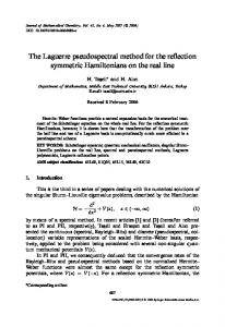
In this section we describe the results from a series of numerical experiments that show the potential of the methods just proposed. To that end, we have developed a numerical code that implements the techniques previously described. This code is based on the C language and the use of the GNU Scienti�c Library [73], mainly for calculations with special functions, and the FFTW library [69] for performing FFTs. In the implementation of the physical domain in the numerical code we have adopted a comoving tortoise coordinate: rc∗ = r∗ − rp∗ . In this way, the particle location (and we emphasize again that we only deal with circular orbits) is always rc∗ = 0. The �rst test we have performed is to study the evolution of a simple wave equation using the formulation and methods described in the previous sections. This case corresponds to: ` = m = 0, M = 0 (which implies V` = 0), and q = 0 (that is, no source, S`m = 0). The test consists in following the propagation of an initial Gaussian packet in a multidomain grid and to study the convergence of the numerical scheme as the number of collocation points per subdomain, N , increases. In Figure 2, we show a convergence plot for a simulation that uses two subdomains, r∗ − rp∗ ∈ [−550 M, 0] ∪ [0, 550 M ], connected by the penalty method as described in subsection III C. The truncation error has been computed in the subdomain where the Gaussian packet is present at a chosen time. As one can see, the truncation error, estimated as the absolute value of the last spectral coe�cient, |aN |, decreases exponentially with the number of collocation points, as expected in the PSC method for smooth solutions. The same convergence follows for an initial Gaussian wave packet propagating on a Schwarzschild background, that is, for the case in which only S`m = 0. This is expected as the mathematical structure of the equation is essentially the same. The additional ingredient is the excitation of quasinormal modes of the black hole by the initial wave packet. When we introduce the SCO, i.e. the particle, the situation is conceptually di�erent. If we think in global terms, the presence of the particle implies that the global solution (the solution in the whole computational domain) will not be smooth. Hence, we cannot expect exponential convergence for the solution of our problem. However, as we have argued above, our multidomain framework avoids the presence of Dirac delta distributions in the equations by locating the particle in the interface between subdomains. Then, the presence of the particle enters through boundary conditions, actually matching conditions between subdomains. Therefore, at each subdomain we will have a smooth solution, and hence we
FIG. 2: This �gure shows the dependence of the truncation error (estimated by the logarithm of the absolute value of the last spectral coe�cient, log10 |aN |, associated with the �eld ψ ) with respect to the number of collocation points. This error corresponds to an snapshot of the evolution of the classical wave equation, for an initial condition given by a moving Gaussian packet. The data indicates the exponential convergence of the numerical method.
expect our numerical solution to converge exponentially towards it. In our numerical experiments with a particle (remember we restrict ourselves to the case of circular orbits), we take zero initial data, that is ∗ m ∗ ψ`m (to , r∗ ) = φm ` (to , r ) = ϕ` (to , r ) = 0 .
(66)
This initial data is obviously not consistent with Einstein's equations, and as a consequence the evolution produces an initial unphysical burst. We have to wait until this unphysical feature propagates away in order to analyze the solution and obtain physically relevant results. In Figure 3 we show snapshots of the evolution of a scalar charged particle in circular motion at the Last Stable Orbit (LSO), in principle the most demanding case (in Schwarzschild the LSO is located at rp = 6 M ). The �gure includes details of the di�erent m variables, (ψ`m , φm ` , ϕ` ) for ` = m = 2, near the particle location. These snapshots illustrate the ability of our method to capture the structure of the solution near the particle, in particular the ability of resolving the jump in the radial derivative of the �eld (snapshot on the right in Figure 3). In order to further validate our numerical code, we have performed simulations with the particle at the LSO changing the number of collocation points, while leaving the number of subdomains �xed. In this way we have checked that our method can achieve the exponential convergence in each individual subdomain. In Figure 4 we show a convergence plot obtained from simulations that use four subdomains: r∗ − rp∗ ∈ [−550 M, −20 M ] ∪ [−20 M, 0]∪[0, 20 M ]∪[20 M, 550 M ]. The number of collocation points, N , is the same at each subdomain, and in this way we have more resolution near the particle,
10
FIG. 3: We show snapshots of the evolution of the scalar charged particle in circular motion at the LSO for the mode ` = m = 2. These simulations used 12 subdomains and 50 collocation points per subdomain. They show the evolution of the variables m ψ`m (left), φm ` (center), and ϕ` (right), after a substantial time has passed and a number of wave cycles have been generated. In particular they show how the jump in the radial derivative of the �eld Φm ` is resolved (this information is encoded in the variable ϕm ` ) in this multidomain computational framework.
where it is most needed. The �gure shows that indeed our numerical scheme has exponential convergence.
FIG. 4: This �gure shows the dependence of the truncation error (log10 |aN |) with respect to the number of collocation points for simulations of circular motion at the LSO (rp = 6 M ) corresponding to the ` = m = 2 mode, in particular for the �eld ψ22 . The data, taken from the subdomain r∗ − rp∗ ∈ [0, 20 M ] indicates the exponential convergence of the numerical method.
The multidomain feature of our method is useful for another important reason, namely computational cost. It is not the same having N points in D domains that having N · D points in one single domain. This is an important fact to be considered in a situation where the need for resolution comes only from some isolated regions of the computational domain. This is what happens in our problem and the type of multidomain structure can have dramatic consequences in the calculations. First of all, for computations in a given time step, the �rst option involves less calculations. Second, from the evolution point of view, in the PSC method, the Courant-Friedrichs-Lax (CFL) condition on the allowed size of the time step, ∆t, is more stringent than in Finite Di�erences (FD) schemes. For the PSC method the maximum allowed time step is ∆tCF L ∼ π 2 |rR∗ − rL∗ |/(4N 2 ) (this is set by the minimum distance between two collocation points,
which occurs at the boundaries of the subdomains [61]), that is, it goes like 1/N 2 with respect to the number of collocation points, whereas in FD schemes it goes like 1/N . Then, dividing the domain in subdomains can help in having a bigger ∆tCF L . In addition, the multidomain scheme can be seen as a way of adaptivity, in the sense that we can construct small subdomains for the regions that need to be well resolved, essentially near the particle, and large subdomains for the regions that do not need to have high resolution, essentially far away from the particle. In order to illustrate how the multidomain feature of our numerical framework works, we have performed simulations with a �xed number of collocation points but changing the number of subdomains. The aim is to show how the solution improves by adding new subdomains. In our simulations, the most demanding region for resolution is clearly near the particle. Apart from this we have the waves leaving the particle location and going both towards the horizon and towards spatial in�nity. These waves are in principle easy to resolve, but for modes with high ` and m we have that the source term oscillates like q exp{im Ωp (t−to )} (where Ωp = M/rp3 is the coordinate angular velocity of the particle), and hence the wavelength gets reduced so that we have many more waves that for low m. These waves are moving away and need to be resolved. In Figure 5 we show snapshots of evolutions with 50 collocation points per subdomain, but with di�erent number of subdomains, namely from 2 to 16 subdomains (half of them to the left of particle and the other half to the right). The �gure shows the mode ` = 10 and m = 6 (so that the period of the waves is π/(3Ωp )) for the three �elds (ψ, φ, ϕ). We can see how for few subdomains the waves are unresolved, and that as we increase the number of subdomains the solution converges. Therefore, the multidomain structure is a very useful tool to achieve accurate results with a reasonable computational cost. The key point is to realize what is the optimal number of subdomains, their size, and their distribution over the whole computational domain. Given that in our case the period of the waves changes with the harmonic num-
11 ber m, the optimal strategy for setting the subdomain will depend on it. However, since the main aim of this work is to show the principal ingredients of the method and to illustrate its performance, we have not explored the possibility of changing the subdomain structure as m changes. However, this is something that should be done for optimizing the computational cost in the case of systematic calculations of the self-force. In this sense, it would be convenient to have a deep understanding of the computational parameter space in order to automatically adapt these parameters to the physical parameters and optimize in this way the calculations. This would require an extensive investigation that will be done and presented elsewhere. The next step in the validation of the code is to compute the components of the self-force acting on the charged scalar particle moving in circular geodesics around a nonrotating black hole. This is the goal of this numerical scheme, that is, to provide accurate computations of the self-force with reasonable computational cost. The calculation of the self-force require to compute the evolution of the real and imaginary parts [note that the source term in the evolution equation (10) is complex and hence both the real and imaginary parts are needed] of the (`, m) harmonic components of Φm ` . Since Φ is a real scalar we have that for each (`, m) the rela¯ −m = (−1)m Φm holds and hence we do not need tion Φ ` ` to compute the modes with m < 0. Given that we need to truncate the sum over (`, m) at a given `max , the total number of evolutions that we need to run for a single selfforce calculation is Nevolutions = [(`max + 1)(`max + 2)/2], where here the brackets denote the the nearest integer to the argument. For the particular case `max = 20, a typical case in our calculations, we need to perform Nevolutions = 231 evolutions. In Table I we present the results of the computations of the self-force vector (actually of the gradient of the regular scalar �eld) acting on a scalar particle in circular (geodesic) motion around a black hole at the following radii: r/M = 6, 7, 8, 10, 14, and 20. For these simulations we have used our multidomain framework with subdomains that contain 50 collocation points. We have used the same number of subdomains to the right and to the left of the particle. The size of these subdomains is typically ∆r∗ = 20, specially those near the particle. As we get far away enough from the particle towards the boundaries (typically at r∗ = ±(500−700)M ), the size of the subdomains is increased since we need less resolution in those regions. The total number of subdomains that we have used ranges from 12 − 34. We have observed that at some point increasing the number of subdomains (maintaining the size of r∗ = 20M ) does not change signi�cantly the results. Another important point to mention is the fact that we are computing the self-force right at the particle location. But since the particle is at the interface between two subdomains, we obtain two values of the self-force components, one from the subdomain to the left [let us call it Ωa as in equation (47)],
R,− = ΦR (r∗ ), and the other one from the subdomain Φα α a,R ∗ to the right (Ωa+1 ), ΦRα,+ = ΦRα (ra+1,L ). This also pro-
vides us with a test of the numerical calculations as both values have to agree to a good gegree of precision. In Table I we show our results and compare them with two types of calculations in the literature: (i) Calculations based on a time-domain method that uses a characteristic formulation of the scalar �eld equations [36]; (ii) calculations based on a frequency-domain method [74]. As we can see, we can get a good numerical approximation to the self-force components using a modest amount of computational resources. It is important to mention that these computations have a relatively low computational cost (relative to the computational cost of time-domain simulations of this sort). The average time for a full selfforce calculation of the type just described in a computer with two Quad-Core Intel Xeon processors at 2.8 GHz is always in the range 20 − 30 minutes. V.
CONCLUSIONS AND DISCUSSION
In this paper we have introduced a new time-domain technique for the simulations of EMRIs. The main ingredient of the method is to use a multi-domain framework in which the SCO, described as a point-like object, is located at the interface between two subdomains. In this way we have shown that this technique enjoys the exponential convergence property of the PSC method and its accuracy and, at the same time, it is also an e�cient method to make time-domain computations of the selfforce. We have shown that we can achieve a good accuracy in this computations by using a relatively low number of collocation points. In this sense, the multidomain framework allows us to locate more collocation points in the region where they are most needed, i.e. around the particle, by choosing appropriately the number of subdomains, and their size and location. Another positive property of our numerical scheme is that it can be easily parallelized to be used in supercomputers, as we can assign the work of each subdomain to di�erent CPUs. The only information that we need to communicate is the one necessary to satisfy the matching conditions between subdomains. The calculations performed for this paper show the potential of this technique for the description of EMRIs. These results still leave room for improvement as we have not explore yet the full parameter space of the numerical method (number of collocation points per subdomain, number and distribution of subdomains, parameters of the spectral �lter, penalty parameters, etc), which is wide enough. In this regard, it would be convenient to be able to adjust the computational parameters to the physical parameters of each mode in an automatic way. In addition to this, there are several additions/modi�cations to the present numerical framework that may improve the present accuracy and e�ciency of the calculations, some of which we will investigated in future calculations by the
12
FIG. 5: We show here three plots of an snapshot of the evolution of the scalar charged particle in circular orbital motion at the LSO for the mode ` = 10 and m = 6. Each plot shows di�erent evolutions of the variables ψ (left), φ (center), and ϕ (right), for a �xed number of collocation points (N = 50), but for di�erent numbers of subdomains (D = 2, 6, 10, 16). In this we can see how increasing the number of subdomains leads to a better accuracy (we can see how the waves get better resolved and the solution converges as we increase the number of subdomains) with a much less computational cost as if we would have increase the number of collocation points in a single domain computational framework. TABLE I: In this table we show the values of the regular �eld at the particle location, (ΦRα,− , ΦRα,+ )a , computed at ϕp = 0. These results are obtained for for `max = 20, N = 50, and D = 12 − 36. The minimum size of the subdomains, as measured in terms of the tortoise coordinate is ∆r∗ = 20M , which corresponds to the subdomains near the particle location. The table shows our numerical results for di�erent circular orbits (r/M = 6, 7, 8, 10, 14, and 20) and the relative errors with respect to the results obtained with a time-domain method in [47], and with a frequency-domain method in [74] and [36]. r(M )
6 7 8 10 14 20
Component of ΦRα
Estimation using the PSC Method
,− ,+ (ΦR , ΦR ) (3.60777, 3.60778) · 10−4 t t ,− R,+ ) (1.67364, 1.67362) · 10−4 (ΦR , Φ r r ,− R,+ −3 (ΦR ϕ , Φϕ ) (−5.30422, −5.30438) · 10 R ,− R ,+ −4 (Φt , Φt ) (1.76638, 1.76639) · 10 ,− ,+ (ΦR , ΦR ) (7.84007, 7.84001) · 10−5 r r ,− R,+ ) (−3.2730, −3.2733) · 10−3 (ΦR , Φ ϕ ϕ ,− ,+ (ΦR , ΦR ) (9.76454, 9.76457) · 10−5 t t R ,− R ,+ (Φr , Φr ) (4.0835, 4.0832) · 10−5 R ,− R ,+ (Φϕ , Φϕ ) (−2.2115, −2.2108) · 10−3 ,− ,+ (ΦR , ΦR ) (3.74362, 3.74363) · 10−5 t t ,− R,+ ) (ΦR , Φ (1.3804, 1.3801) · 10−5 r r R ,− R ,+ (Φϕ , Φϕ ) (−1.1860, −1.1858) · 10−3 ,− ,+ (ΦR , ΦR ) (9.176912, 9.176914) · 10−6 t t R ,− R ,+ (Φr , Φr ) (2.7269, 2.7266) · 10−6 ,− R,+ ) (−4.8383, −4.8389) · 10−4 (ΦR , Φ ϕ ϕ ,− ,+ (ΦR , ΦR ) (2.08859, 2.08858) · 10−6 t t R ,− R ,+ (Φr , Φr ) (4.9444, 4.9440) · 10−7 R ,− R ,+ (Φϕ , Φϕ ) (−1.92449, −1.92436) · 10−4
Estimation from Error relative to Error relative to Frequency-domain Frequency-domain Time-domain calculations in [74] and [36] calculations in [74] and [36] calculations in [47] 3.609072 · 10−4 (0.03, 0.03) % (0.12, 0.12) % 1.67728 · 10−4 (0.2, 0.2) % (0.18, 0.18) % −5.304231 · 10−3 (4 · 10−4 , 10−3 ) % (6 · 10−4 , 10−3 ) % 7.85067 · 10−5
(0.13, 0.13) %
4.08250 · 10−5
(0.02, 0.01) %
1.37844 · 10−5
(0.14, 0.12) %
2.72008 · 10−6
(0.25, 0.24) %
4.93790 · 10−7
(0.13, 0.12) %
a We show the values of the gradient of the regular �eld instead of the components of the self-force for the sake of comparing with other results in the literature.
present authors. We list here some of them: (i) Compacti�cation of the computational domain. We can change the mapping between the spectral and physical domains incorporating the two in�nities (the horizon location at rH∗ → −∞ and spatial in�nity at rI∗ → ∞) into the calculation. In practice, this mapping only would need to be performed in the �rst and last subdomains. By doing this, the outgoing boundary conditions (32) would be exact instead of approximate as they are know. An alternative to this could be to improve the boundary conditions by analyzing the solution near the two in�nities, like for instance in [75] in a frequency domain framework.
(ii) Reduction of the time step. As we have mentioned before, the PSC method has a more strict CFL condition as a FD scheme, namely ∆t ∼ N −2 versus ∆t ∼ N −1 . This is because of high density of collocation points near the boundaries and the fact that the minimum time step come from the minimum separation between points. A way of changing this is again to change the mapping between the spectral and physical domains. One known way of doing this is the modi�cation introduced by Koslo� and Tal-Ezer [76], which was shown to lead to a time step restriction like in the FD case, that is ∆t ∼ N −1 . (iii) Richardson extrapolation. In our calculations we have
13 computed harmonic components of the scalar �eld, Φm ` , up to a certain `max , in this work `max = 15 − 20. In other words, we have truncated the expansion in spherical harmonics. We can try to improve the �nal numerical results for the scalar �eld and derived quantities, like the self-force, by pro�ting from our analytical knowledge of the expansions in inverse powers of the harmonic number `. This can be done using numerical techniques based on the Richardson extrapolation, like in [35], which can provide an estimation of the di�erent quantities of interest as `max → ∞. Beyond the case studied in this paper, circular orbits of a charged scalar particle, we will study in the future how to extend our time-domain computational framework in order to include generic (eccentric) orbits. The main dif�culty is obviously to deal with a particle moving the radial direction as our present framework assumes that it is located at a �xed value (circular motion). There are several ways in which we can attack this problem. One is to try to implement some type of moving grid technique (as it was done in a similar situation in [46]), but the reconstruction of the grid at every time step could increase signi�cantly the computational cost of the evolution. Another possibility is to try to make a change of coordinates to coordinates comoving with the particle, so that the techniques presented in this paper can be implemented in a straightforward way. On the other hand, we expect that MBHs sitting at galactic centers will have considerable spins (a/M ∼ 0.7 or bigger, where a is the Kerr spin parameter) and hence the MBH should be described by the Kerr metric instead of the Schwarzschild metric. This means to have a less symmetric background, instead of the spherical symmetry of Schwarzschild just the axisymmetry of Kerr. In that case one can separate the dependence on the azimuthal angle and is left with 2 + 1 wave-type equations with singular terms. The main di�culty in this case is that each m-mode (coming from the separation of the azimuthal angle) diverges logarithmically at the particle location. Then, before trying to transfer the techniques presented in this paper to the Kerr case, one has to apply before a regularization procedure as it has been done in [48, 54, 59]. Apart from this, we expect that most of the methods presented in this paper will be helpful in achieving e�cient simulations of EMRIs in the case of a spinning MBH.
predoctoral FPU fellowship of the Spanish Ministry of Science and Innovation (MICINN). Financial support from the Spanish Ministry of Science and Education contract ESP2007-61712 is gratefully acknowledged. This research has been partly performed using the resources of the Centre de Supercomputació de Catalunya (CESCA). APPENDIX A: SPECIAL FUNCTIONS USED IN THIS WORK
Here, we summarize the main conventions used for the special functions involved in calculations of this paper. 1.
Spherical Harmonics
The expression we use for the scalar spherical harmonics is: s Y`m (θ, ϕ)
=
2` + 1 (` − m)! m P (cos θ)eimϕ , 4π (` + m)! `
where P`m are the associated Legendre polynomials [we use the same expressions as in [67], equations (8.6.6) and (8.6.18)] (−1)`+m d`+m (1 − x2 )m/2 `+m (1 − x2 )` , (A2) ` 2 `! dx where ` is a non-negative integer and m is an integer restricted to the following range: m ∈ (−` , −` + 1 , . . . , ` − 1 , `) . P`m (x) =
2.
Chebyshev Polynomials
The Chebyshev polynomials can be expresses as follows: � Tn (X) = cos n cos−1 (X) ,
We would like to thank Leor Barack, José Luis Jaramillo and Eric Poisson for helpful discussions and encouragement. CFS acknowledges support from the Ramón y Cajal Programme of the Ministry of Education and Science of Spain and by a Marie Curie International Reintegration Grant (MIRG-CT2007-205005/PHY) within the 7th European Community Framework Programme. PCM is supported by a
(A3)
and are de�ned in the interval [−1, 1] with |Tn (X)| ≤ 1, where n is the degree of the polynomial. Chebyshev polynomials are orthogonal in the continuum in the following sense: Z
1
(Tn , Tm ) = −1
Acknowledgments
(A1)
√
dX πc Tn (X) Tm (X) = n δnm , 2 2 1−X
(A4) where the coe�cients cn are given in equation (45). The set of collocation points for the spatial discretization of our PDEs by means of the PSC method are the extrema of the Chebyshev polynomials, together with the end points X = ±1 [that is, the zeros of the polynomial given in equation 34)]. These points form, in the interval [−1, 1], a Chebyshev-Lobatto collocation grid. The cardinal functions associated with them are (i = 0, . . . , N ): Ci (X) =
(1 − X 2 )TN0 (X) . (1 − Xi2 )(X − Xi )TN00 (Xi )
(A5)
14 Once this set of collocation points is adopted, and taking into account the properties of the Gauss-LobattoChebyshev quadratures (see, e.g. [61]), the Chebyshev polynomials have another orthogonality relation, this time in the discrete, in the following sense (n, m = 0, . . . , N ): [Tn , Tm ] =
N X
wi Tn (Xi ) Tm (Xi ) = νn2 δnm ,
(A6)
i=0
where wi are the weights associated with the ChebyshevLobatto grid, wi = π/(N c¯i ), and where the c¯i 's are normalization coe�cients given by ( c¯i =
2 for i = 0, N , 1 otherwise .
(A7)
Finally, the constants νn in (A6) are given by νn2 = π¯cn /2. On the other hand, introducing a new variable, X = cos θ, the Chebyshev polynomials look like Tn (cos θ) = cos(nθ) .
APPENDIX B: SPECTRAL FILTER
In order to reduce the spurious high-frequency components of our numerical solutions, we apply a spectral
[2] [3] [4] [5] [6] [7] [8] [9] [10] [11] [12] [13]
FFT
http://www.esa.int/science/lisa, http://lisa.jpl.nasa.gov.
Filter
FFT
˜ }, {U i } −→ {an } −→ {˜ an } −→ {U i
(B1)
where {U i } are the values of the solutions at the collocation points after the RK step; {an } are their corresponding spectral components; {bn } are the �ltered spectral ˜ } are the �ltered values of the socomponents; and {U i lution at the collocation points. The exponential �lter is de�ned by its action on the spectral coe�cients {an } to yield the spectral coe�cients {bn }. This action is given by ˜n = σ a
�n� N
an ,
(B2)
where σ(n/N ) is the exponential �lter
(A8)
Then, an expansion in Chebyshev polynomials can be mapped to a cosine expansion.
[1] LISA,
�lter of the exponential type to the solution after every time step, that is, after every full RK step. The scheme for the action of the spectral �lter is
σ
�n� N
( =
1 h i for 0 6 n 6 Nc , (B3) n−N exp −α( N −Nc )γ for Nc < n ≤ N , c
where Nc is the cut-o� mode number, γ is the order of the �lter (typically chosen to be of the order of the number of collocation points, N ), and α is the machine accuracy parameter, which is related to the machine accuracy, �M , by α = − ln �M .
[14] S. A. Hughes, S. Drasco, E. E. Flanagan, and J. Franklin, Phys. Rev. Lett. 94, 221101 (2005), gr-qc/0504015. J. R. Gair, L. Barack, T. Creighton, C. Cutler, S. L. [15] S. Drasco and S. A. Hughes, Phys. Rev. D73, 024027 Larson, E. S. Phinney, and M. Vallisneri, Class. Quant. (2006), gr-qc/0509101. Grav. 21, S1595 (2004), gr-qc/0405137. [16] N. Sago, T. Tanaka, W. Hikida, and H. Nakano, Prog. C. Hopman and T. Alexander, Astrophys. J. 645, L133 Theor. Phys. 114, 509 (2005), gr-qc/0506092. (2006), astro-ph/0603324. [17] K. Ganz, W. Hikida, H. Nakano, N. Sago, and T. Tanaka S. Sigurdsson and M. J. Rees (1996), astro-ph/9608093. (2007), gr-qc/0702054. P. Amaro-Seoane et al., Class. Quant. Grav. 24, R113 [18] Y. Mino, Phys. Rev. D67, 084027 (2003), gr-qc/0302075. (2007), astro-ph/0703495. [19] A. Pound, E. Poisson, and B. G. Nickel, Phys. Rev. D72, D. A. Brown et al., Phys. Rev. Lett. 99, 201102 (2007), 124001 (2005), gr-qc/0509122. gr-qc/0612060. [20] A. Pound and E. Poisson, Phys. Rev. D77, 044012 I. Mandel, D. A. Brown, J. R. Gair, and M. C. Miller (2008), 0708.3037. (2007), 0705.0285. [21] Y. Mino, Phys. Rev. D77, 044008 (2008), 0711.3007. Advanced LIGO, http://www.ligo.caltech.edu/advLIGO. [22] T. Hinderer and E. E. Flanagan (2008), 0805.3337. Advanced VIRGO, http://wwwcascina.virgo.infn.it/advirgo [23]. Y. Mino, M. Sasaki, and T. Tanaka, Phys. Rev. D55, L. S. Finn and K. S. Thorne, Phys. Rev. D62, 124021 3457 (1997), gr-qc/9606018. (2000), gr-qc/0007074. [24] T. C. Quinn and R. M. Wald, Phys. Rev. D56, 3381 E. Poisson, Living Rev. Relativity 7, 6 (2004), (1997), gr-qc/9610053. gr-qc/0306052, URL http://www.livingreviews.org/ [25] S. Detweiler and B. F. Whiting, Phys. Rev. D67, 024025 lrr-2004-6. (2003), gr-qc/0202086. T. Tanaka, Prog. Theor. Phys. Suppl. 163, 120 (2006), [26] S. E. Gralla and R. M. Wald, Class. Quant. Grav. 25, gr-qc/0508114. 205009 (2008), 0806.3293. K. Glampedakis, Class. Quant. Grav. 22, S605 (2005), [27] A. O. Barut, Electrodynamics and Classical Theory of gr-qc/0509024. Fields and Particles (Dover, New York, 1980).
15 [28] J. D. Jackson, Classical Electrodynamics (John Wiley & Sons, New York, 1999), 3rd ed. [29] L. Barack and A. Ori, Phys. Rev. D61, 061502 (2000), gr-qc/9912010. [30] L. Barack, Phys. Rev. D62, 084027 (2000), grqc/0005042. [31] L. Barack, Phys. Rev. D64, 084021 (2001), grqc/0105040. [32] Y. Mino, H. Nakano, and M. Sasaki, Prog. Theor. Phys. 108, 1039 (2003), gr-qc/0111074. [33] L. Barack, Y. Mino, H. Nakano, A. Ori, and M. Sasaki, Phys. Rev. Lett. 88, 091101 (2002), gr-qc/0111001. [34] L. Barack and A. Ori, Phys. Rev. D66, 084022 (2002), gr-qc/0204093. [35] S. Detweiler, E. Messaritaki, and B. F. Whiting, Phys. Rev. D67, 104016 (2003), gr-qc/0205079. [36] R. Haas and E. Poisson, Phys. Rev. D74, 044009 (2006), gr-qc/0605077. [37] T. Regge and J. A. Wheeler, Phys. Rev. 108, 1063 (1957). [38] M. Davis, R. Ru�ni, and J. Tiomno, Phys. Rev. D 5, 2932 (1972). [39] S. L. Detweiler, Astrophys. J. 225, 687 (1978). [40] S. L. Detweiler and E. Szedenits, Jr., Astrophys. J. 231, 211 (1979). [41] C. Cutler, D. Kenne�ck, and E. Poisson, Phys. Rev. D50, 3816 (1994). [42] E. Poisson, Phys. Rev. D52, 5719 (1995), gr-qc/9505030. [43] E. Poisson, Phys. Rev. D55, 7980 (1997). [44] K. Martel, Phys. Rev. D69, 044025 (2004), grqc/0311017. [45] L. Barack and C. O. Lousto (2005), gr-qc/0510019. [46] C. F. Sopuerta and P. Laguna, Phys. Rev. D73, 044028 (2006), gr-qc/0512028. [47] R. Haas, Phys. Rev. D75, 124011 (2007), 0704.0797. [48] I. Vega and S. Detweiler, Phys. Rev. D77, 084008 (2008), 0712.4405. [49] L. Barack and N. Sago, Phys. Rev. D75, 064021 (2007), gr-qc/0701069. [50] L. M. Burko and G. Khanna, Europhys. Lett. 78, 60005 (2007), gr-qc/0609002. [51] P. A. Sundararajan, G. Khanna, and S. A. Hughes, Phys. Rev. D76, 104005 (2007), gr-qc/0703028. [52] P. A. Sundararajan, G. Khanna, S. A. Hughes, and S. Drasco, Phys. Rev. D78, 024022 (2008), 0803.0317. [53] C. F. Sopuerta, P. Sun, P. Laguna, and J. Xu (2005), gr-qc/0507112. [54] L. Barack and D. A. Golbourn, Phys. Rev. D76, 044020 (2007), 0705.3620. [55] S. Brandt and B. Bruegmann, Phys. Rev. Lett. 78, 3606 (1997), gr-qc/9703066. [56] M. Campanelli, C. O. Lousto, P. Marronetti, and Y. Zlochower, Phys. Rev. Lett. 96, 111101 (2006), grqc/0511048. [57] J. G. Baker, J. Centrella, D.-I. Choi, M. Koppitz, and J. van Meter, Phys. Rev. Lett. 96, 111102 (2006), grqc/0511103. [58] L. Barack, D. A. Golbourn, and N. Sago, Phys. Rev. D76, 124036 (2007), 0709.4588. [59] C. O. Lousto and H. Nakano, Class. Quant. Grav. 25, 145018 (2008), 0802.4277. [60] P. Canizares and C. F. Sopuerta, in Proceedings of the 7th International LISA Symposium (2008), 0811.0294. [61] J. P. Boyd, Chebyshev and Fourier Spectral Methods
(Dover, New York, 2001), 2nd ed. [62] P. Grandclement and J. Novak, Living Rev. Relativity 12, 1 (2009), 0706.2286, URL http://www. livingreviews.org/lrr-2009-1. [63] J.-H. Jung, G. Khanna, and I. Nagle (2007), 0711.2545. [64] S. E. Field, J. S. Hesthaven, and S. R. Lau (2009), 0902.1287. [65] T. C. Quinn, Phys. Rev. D62, 064029 (2000), grqc/0005030. [66] L. Barack and A. Ori, Phys. Rev. D67, 024029 (2003), gr-qc/0209072. [67] M. Abramowitz and I. A. Stegun, Handbook of Mathe[68] [69] [70] [71]
[72] [73]
[74] [75] [76]
matical Functions with Formulas, Graphs, and Mathematical Tables (Dover, New York, 1972). B. Gustafsson, H. Kreiss, and J. Oliger, Time dependent problems (John Wiley & Sons, New York, 1995). M. Frigo and S. G. Johnson, Proceedings of the IEEE 93, 216 (2005), special issue on "Program Generation, Optimization, and Platform Adaptation". J. C. Butcher, Numerical Methods for Ordinary Di�erential Equations (John Wiley & Sons, Chichester, 2008), 2nd ed. W. H. Press, B. P. Flannery, S. A. Teukolsky, and W. T. Vetterling, Numerical Recipes: The Art of Scienti�c Computing (Cambridge University Press, Cambridge, 1992). J. S. Hesthaven, Applied Numerical Mathematics 33, 23 (2000). M. Galassi, J. Davies, J. Theiler, B. Gough, G. Jungman, M. Booth, and F. Rossi, GNU Scienti�c Library Reference Manual (Network Theory Ltd., Bristol, 2006), 2nd ed. L. M. Diaz-Rivera, E. Messaritaki, B. F. Whiting, and S. Detweiler, Phys. Rev. D70, 124018 (2004), grqc/0410011. L. Barack, A. Ori, and N. Sago, Phys. Rev. D78, 084021 (2008), 0808.2315. D. Koslo� and H. Tal-Ezer, Journal of Computational Physics 104, 457 (1993).