An Effective Algorithm for Implementing Perfectly. Matched Layers in Time-Domain Finite-Element. Simulation of Open-Region EM Problems. Dan Jiao, Member ...
IEEE TRANSACTIONS ON ANTENNAS AND PROPAGATION, VOL. 50, NO. 11, NOVEMBER 2002
1615
An Effective Algorithm for Implementing Perfectly Matched Layers in Time-Domain Finite-Element Simulation of Open-Region EM Problems Dan Jiao, Member, IEEE, and Jian-Ming Jin, Fellow, IEEE
Abstract—An algorithm is presented to implement perfectly matched layers (PMLs) for the time-domain finite-element (TDFE) simulation of two-dimensional open-region electromagnetic scattering and radiation problems. The proposed algorithm is based on the TDFE solution of a special vector wave equation similar to the one in an anisotropic and dispersive medium. The impact of the PML on the stability of the resultant TDFE solution is studied for a variety of temporal discretization schemes, and it is shown that the proposed algorithm for implementing PML can support unconditionally stable TDFE schemes. Both the totaland the scattered-field formulations are described, and numerical simulations of radiation and scattering problems are presented to validate the proposed PML algorithm for the mesh truncation of the TDFE solution. Index Terms—Electromagnetic scattering, finite-element method (FEM), numerical analysis, numerical stability, time domain analysis.
I. INTRODUCTION
N
UMERICAL simulations of open-region wave propagation problems based on partial differential equation (PDE) solvers usually require an absorbing boundary condition (ABC) to properly truncate the computational domain. Among a variety of ABCs developed in the past decades, the perfectly matched layer (PML) [1]–[13] is a popular choice since it allows for the absorption of outgoing waves with any polarizations and at any frequencies and angles of incidence. The PML can be formulated by using field splitting [1]–[3], coordinate stretching [4]–[7], or by constructing anisotropic permittivity and permeability tensors [8]–[11]. These formulations are shown to be equivalent. The PML was utilized for the grid truncation of the finite-difference time-domain (FDTD) method [1]–[4], [9], [12]. In particular, Roden and Gedney [13] proposed recently an approach to implement PML in the FDTD based on a recursive convolution. The PML was also used for the mesh truncation in the frequency-domain finite-element method (FDFEM) [5], [8], [10], [11]. To the best of the authors’ knowledge, the PML has not been applied to the time-domain finite-element method (TDFEM) because of difficulties associated with the modeling of both dispersive and anisotropic medium. Manuscript received February 27, 2001; revised August 30, 2001. This work was supported in part by Grant AFOSR via the MURI Program under Contract F49620–96-1–0025 and in part by a Grant from Sandia National Laboratory. The authors are with the Center for Computational Electromagnetics, Department of Electrical and Computer Engineering, University of Illinois, Urbana-Champaign, Urbana, IL 61801-2991 USA. Digital Object Identifier 10.1109/TAP.2002.803987
Recently, a considerable amount of effort has been devoted to the development of time-domain numerical techniques, as these techniques permit the generation of broadband data and the modeling of nonlinear devices. A variety of TDFEM approaches have been proposed [14]–[30]. One class of approaches directly solves Maxwell’s equations [14]–[22]. These approaches usually operate in a leapfrog fashion similar to the FDTD method, which does not leverage our extensive knowledge of frequency-domain finite-element solvers. Another class of TDFEM approaches tackles the second-order vector wave equation [23]–[29]. These approaches have a disadvantage in that they require the solution of a matrix equation at each time step. However, this problem can be eliminated by employing orthogonal vector basis functions [28], [31], which render a diagonal mass matrix, and hence a purely explicit scheme. The problem can also be mitigated by adopting higher order vector basis functions [32] to expedite the TDFEM numerical convergence. An important issue in the finite-element solution of open-region problems is the treatment of the artificial truncation boundary. One approach is to represent the exterior field using a boundary integral (BI) expression. This leads to the FE-BI method (see [33] and references therein). This approach was initially developed within the context of frequency domain solvers. It has been recently extended to the time domain [32], [34]. The BI approach is numerically exact, and it allows the truncation boundary to take on any shape and to be placed to the object as close as possible. However, the evaluation of the BIs is computationally expensive. Although this evaluation can be accelerated by invoking the multilevel plane-wave time-domain (PWTD) algorithm [32], [35] its efficiency benefits mostly the analysis of electrically large and concave objects. For convex objects, the local ABCs such as the PML, often prove to be more efficient. However, unlike the situation in the FDTD method, the development of ABCs, especially the PMLs for TDFEMs, has not received much attention. To date, only firstand second-order ABCs have been implemented [36]–[38]. The major difficulty in the implementation of PMLs in the framework of TDFEM lies in the modeling of both dispersive and anisotropic medium. A recent work [39] provides a guideline for the TDFEM modeling of dispersive media. By following this guideline and incorporating the correct handling of anisotropic media, an algorithm is developed in this paper for the PML implementation in the TDFEM. The proposed algorithm is based on seeking the TDFEM solution of a special
0018-926X/02$17.00 © 2002 IEEE
1616
Fig. 1.
IEEE TRANSACTIONS ON ANTENNAS AND PROPAGATION, VOL. 50, NO. 11, NOVEMBER 2002
Illustration of the solution domain truncated by the PML.
vector-wave equation similar to the one in an anisotropic and dispersive medium. The approach to handle both dispersive and anisotropic medium is addressed. The impact of the PML on the stability of the entire TDFEM procedure is analyzed. It is shown that the proposed algorithm can support unconditionally stable TDFEM schemes. Since the proposed PML implementation is similar to that for an anisotropic and dispersive medium, it can readily be incorporated into the existing TDFEMs. Numerical results are presented to demonstrate its validity. In this paper, the proposed algorithm for PML implementation in the TDFEM is described in Section II. Both the total- and scattered-field formulations are presented. Section III examines the stability of the resulting TDFEM-PML numerical scheme. Section IV demonstrates the capabilities and accuracy of the proposed TDFEM-PML through a host of examples. Finally, Section V relates our conclusions.
Fig. 2. Magnetic field H at � source.
= 00:23^x + 0:002^y m radiated by a line
to terminate the PML at . Inside the PML, the fields and satisfy the following modified Maxwell’s equations [1]
(1) . Obviously, inside , (1) reduces in which to the original Maxwell’s equations. Hence, (1) is valid for both and the PML region. By eliminating and from (1), are constant within each element, and assuming , , and we obtain the second-order vector wave equation
II. FORMULATION This section describes the TDFEM-PML formulation for analyzing two-dimensional (2-D) open-region radiation and scattering problems. Throughout, all fields are assumed to be TEz polarized; the proposed scheme, however, also applies to TMz problems with minor modifications. Although the 2-D problem can be solved more easily using the axial component of the magnetic field as the unknown variable, the formulation and implementation are carried out here using the transverse components of the electric field so that the method can be extended to three-dimensional (3-D) vector problems. Consider the problem of modeling the electric field generated by an internal source in the presence of an object residing in a region . To formulate a FE scheme that permits the computation of , we introduce a perfectly to truncate the computational matched layer outside of and , a domain (Fig. 1). In the PML region bounded by is specified for the PML walls perpendicular conductivity is specified for the to the axis; similarly, a conductivity PML walls perpendicular to the axis. A perfectly electric or magnetic conducting wall or any type of ABCs can be used
(2) where stands for the convolution, by
and
are tensors given
(3) and
(4) and denote the Kronecker delta function and the In (4), unit step function, respectively. Equation (2) can also be derived based on the coordinate stretching [4] or the modeling of the PML as an anisotropic medium characterized by frequency-dependent permittivity and permeability tensors [8], [9]. However, despite a certain similarity, it is not identical to the wave equation in an anisotropic medium. To seek the TDFEM solution of (2), we employ Galerkin’s method. Assuming a Dirichlet-type boundary condition on , we obtain a weak-form solution shown in (5), shown at the
JIAO AND JIN: EFFECTIVE ALGORITHM FOR IMPLEMENTING PMLs
1617
bottom of the page, where denotes the whole simulation and the PML region, and domain consisting of both denotes the vector basis function. Expanding the electric field as
, and and can be recursively evaluated as
are matrices whose elements
(15) (6) denoting the total number of expansion functions, and with substituting (6) into (5), we obtain an ordinary differential equation as
denotes the total number of FEs, , , , where are square matrices whose elements are given by
(7) , and
(8) and
(9) denotes the integral over element . Also, In the above, is the unknown vector given by , is the excitation vector given by (10) and
and
are vectors whose elements can be expressed as (11)
In (11), the convolution can be recursively evaluated as (12) in which the field is assumed to be constant within each time step, or
if (12) is used, or
(16) and if (13) is employed. In (15) and (16), permittivity are defined on the triangular element that conductivity contains both th and th edge basis functions; permittivity and conductivity comprise those of the two triangular elements associated with the th edge basis function. The self and consist of two parts contributed by terms in matrices the two-triangular elements associated with the corresponding and are considered as matrices edge basis function. Here, and vary rather than vectors, since the conductivity from element to element in the PML region. The separation of from spatial signature facilitates temporal signature the efficient simulation of dispersion. Otherwise, the matrices relating to the spatial signature require them to be refilled at each time step. The formulation described above is for the radiation case. When the scattering problem is considered, the scattered field should be employed as the working variable in the PML region, as the PML is designed for the absorption of outgoing waves. One approach is to separate the entire computational domain into two regions. In the interior region, the total field formulation is used; whereas in the exterior region, the scattered field formulation is employed. By using this approach, the tangential field continuity can be naturally satisfied at the dielectric interface. However, the total-field and the scattered-field data must be exchanged with each other at the separation boundary, which is computationally cumbersome. In this work, we propose an efficient scattered-field formulation in the entire computational domain. in the entire computational doThe scattered-electric field and the PML remain, which includes both solution domain gion, satisfies
(13) (17) in which a linear variation of the field is assumed for better accuracy. Once the summation is carried out, (7) can be written as (14) sign denotes a matrix operator which scales the where the element in the first matrix by the element residing at the same location in the second matrix, is a constant vector given by
denotes the incident field, and the permittivity at where the right-hand side reverts to its free-space value in the PML region so that the incident source vanishes therein. Assuming a Dirichlet-type boundary condition on , we obtain a weak-form solution as in (18), shown at the bottom of the next page. Apparently, the area integrals related to the incident field in (18) require to be recalculated at each time step, which is computationally expensive. Certainly, we can simplify (18) and
(5)
1618
IEEE TRANSACTIONS ON ANTENNAS AND PROPAGATION, VOL. 50, NO. 11, NOVEMBER 2002
reduce the support of these area integrals from the entire domain to the dielectric-only region. However, the recalculation is inefficient even if the dielectric region is small. This problem can be solved efficiently using the approach proposed as follows: We using the same vector basis funcexpand the incident field , tions as those used to expand the unknown scattered field thus the spatial signature can be decoupled from the temporal signature. The matrices and , which are generated for the use of the scattered field, thereby can be directly applied to the incident field. Hence, the resultant ordinary differential equation becomes
(19) is the projection of the incident field where the vector along the tangential direction of each edge, which is known and can be efficiently updated at each time step. It now remains to choose proper spatial and temporal discretization schemes. For the spatial discretization, the unknown fields can be expanded using the linear edge elements [15], higher order edge elements [40], or orthogonal vector basis functions [28], [34]. For the temporal discretization, we can employ the central difference scheme, the backward difference scheme, and the Newmark method [27], [38]. The forward difference is not used since it leads to definite instability [25], [41]. III. STABILITY ANALYSIS This section analyzes the stability behavior of the TDFEM-PML scheme. Since the stability depends on the temporal discretization, its analysis is addressed for the Newmark method, the backward difference, and the central difference, respectively. A. Newmark Method to Applying the Newmark method [27], [38] with discretize (14) and discarding the contribution from the source, we obtain
By performing the
transform on (20), we obtain
(21) where
represents the
transform of , and (22)
in which (23) is positive definite, its contribution in (14) is Since matrix equivalent to introducing a loss into the system. As shown in [41], the introduction of loss does not affect the stability criterion of the TDFEM procedure. Hence, in the following stability . analysis, we ignore the term related to After removing the second term from (21), we obtain
(24) Instead of analyzing the stability of the above equation, we consider the following one
(25) which is obtained by filling the PML region with the maximum . If the stability of the time-marching process conductivity for (25) is satisfied, the stability of the process for (24) is gurranteed to be satisfied, since the former requires a smaller time step to ensure stability. This is because the terms associated with and , when they are combined with matrix , increase the eigenvalue of the resultant matrix and thereby decrease the maximum allowed time step [41]. Clearly, (25) corresponds to an eigenvalue problem. Denoting as , (25) can be the eigenvalue of matrix system written as
(26)
(20) where time step.
, and
represents the
which is termed as the characteristic equation of (25). Since matrix is positive definite, and matrix is semipositive definite, the eigenvalue is nonnegative. By changing , we trace the roots of (26) in the complex plane. It can be shown that when , the roots are never outside the unit circle. Hence, the maximum value of can reach infinity. As a result, there is no
(18)
JIAO AND JIN: EFFECTIVE ALGORITHM FOR IMPLEMENTING PMLs
1619
constraint on . In other words, using the Newmark method and , the TDFEM procedure together with with the PML can be made unconditionally stable. This is verified by our numerical experiments. B. Backward Difference Applying the backward difference to discretize (14), we obtain
(27) The pertinent
transform becomes
(28) (a)
with matrices
and
defined by
(29) is used. in which the value of at time step in (28), we obtain Removing the term related to
(30) Instead of investigating the above equation to analyze the stability, we consider the following one:
(31) represents the maximum conductivity. The charin which acteristic equation of (31) can be identified as
(32) Obviously, the roots of (32) can never go beyond the unit plane. Hence, using the backward circle in the complex difference, the TDFEM procedure in conjunction with the PML is unconditionally stable. This is also verified by our numerical experiments. C. Central Difference The central difference scheme is a special case of the Newand . Hence, by setting in mark method with (24) to zero, we obtain
(33)
(b) Fig. 3. Electric field scattered by a perfectly conducting cylinder of radius 0.2 m. (a) E at � : x : y m. (b) E at � : x : y m.
= 00 23^ +0 002^
= 00 356^ 00 08^
For a discrete system described by (33), the pole flees from . Following the stability analysis prothe unit circle at posed in [41], we deduce the stability criterion
(34) denotes the spectral radius of matrix . Denote where the maximum time step allowed by the TDFEM in free space , which is equal to [41]. Obviously, the as is smaller than . Hence, in the PML current time step region, the TDFEM numerical scheme requires a smaller time step to ensure stability. However, in the general case that the PML region only accounts for a small fraction in the entire comand putational domain, the matrix is slightly perturbed by
1620
IEEE TRANSACTIONS ON ANTENNAS AND PROPAGATION, VOL. 50, NO. 11, NOVEMBER 2002
(a)
(a)
(b) (b)
E 1 t at � = 00:22^x 0 0:015^y m with t = 00:74^x 0 0:67^y scattered by a dielectric cylinder of radius 0.2 m and a relative permittivity � . (a) � = 4. (b) � = 16. Fig. 4. Electric field
. As a result, the introduction of PML into the TDFEM solution does not affect the stability significantly. IV. NUMERICAL EXAMPLES To validate the proposed PML implementation for the mesh truncation of the TDFEM, we examine several numerical examples here. For all of these examples, the zeroth-order edge element is used to expand the unknown field, and the Newmark is chosen for the temporal discretization method with over the backward difference for its better accuracy and over the central difference for its unconditional stability. The multifrontal method [42]–[44] is used to solve the sparse FEM matrix equation, which is a sparse LU decompostion technique. Note that the factorization is performed only once and that only forward and backward substitutions are needed in each time step,
Fig. 5. Electric field scattered by a dielectric cylinder with radius 0.2 m and . (a) at � : : m with : : . (b) Normalized global rms error versus time.
�
= 16
E 1t
= 00 11^x + 0 054^y
t = 00 81^x + 0 58^y
since matrices , , and are time independent. The first example is the radiation from an infinitely long electric-current line source with the electric current is given by (35) ns and ns. The line source is where placed at the center of the computational domain having a size of 2 m 2 m, which is discretized into 3686 triangular elements, yielding 5609 unknowns. The average edge length is 0.05 m. The PML has a thickness of 0.5 m and is terminated by a perfectly magnetic wall. The conductivity in the PML is assumed to have a quadratic profile, with the maximum conductivity chosen to be or 0.0385 s/m in this example. The profile of this PML and its parameters are also used in the other exm amples. The magnetic field observed at is shown in Fig. 2. Clearly, the simulation results agree very well
JIAO AND JIN: EFFECTIVE ALGORITHM FOR IMPLEMENTING PMLs
1621
(a)
(b) Fig. 6. Scattering from a coated cylinder with radius 0.1 m, coating thickness . (a) Scattered field at � : : m with 0.1 m, and � : : . (b) Total magnetic field H at � : : m.
= 12 t = 00 93^x 00 37^y
E 1t
= 00 196^x + 0 1^y = 0 066^x +0 168^y
with the exact data. It should be noted that during the simulation time, the wave has already traveled 15 times between the source and the truncation boundary. Hence, the PML effectively emulates an unbounded space. The second example is the scattering from a conducting cylinder having a radius of 0.2 m, which is illuminated by a TE-polarized Neumann pulse
has a thickness of 0.5 m and is placed 0.5 m away from the center of the conducting cylinder. A vanished scattered field is enforced at the outer boundary to terminate the PML. The simulation is carried out by using the scattered field formulam tion. The calculated electric fields at m are shown in Fig. 3. Again, the and numerical result is in good agreement with the exact data. The slightly worse agreement in Fig. 3(b) is due to the smaller distance between the observation point and the PML, and thereby, the stronger evanescent waves which cannot be effectively absorbed. The numerical results simulated without using the PML are also shown for comparison in Fig. 3. Next, to examine the capability of the proposed method to handle materials, we simulate a dielectric cylinder having a radius of 0.2 m and a relative permittivity 4. The computational domain, having a same size as in the previous example, is divided into 3606 elements, yielding 5489 unknowns. The cylinder is illuminated by the same TE-polarized Neumann pulse as specified in (36). Fig. 4(a) shows the calculated scatm, together with tered electric field at the exact data and the numerical result generated without using PML. Fig. 4(b) shows the calculated scattered electric field at the same location with the relative permittivity of the cylinder increased to 16. Again, the simulation result agrees very well with the theoretical data. Fig. 5(a) shows the calculated scattered electric field at another observation point, simulated over a longer period. To investigate the global accuracy of the proposed PML implementation, we plot the normalized global rms error with respect to time in Fig. 5(b). The global error was obtained for the calculated field at each edge on the surface of the cylinder. Finally, we simulate a conducting cylinder of radius 0.1 m, coated with a 0.1-m thick dielectric with a relative permittivity equal to 12. The computational region is subdivided into 3564 triangular elements, yielding 5432 unknowns. The incident Neumann pulse is specified in (36). The calculated m and magnetic field at electric field at m are shown in Fig. 6. Next, we change ns and ns, the incident pulse parameters to which increase the maximum incident frequency to 1 GHz. The mesh is correspondingly refined, which yields 22 086 elements and 33 345 unknowns. The maximum conductivity is chosen to be 0.11 s/m. Fig. 7 shows the calculated m and magnetic field at electric field at m. Clearly, the proposed TDFEM-PML scheme correctly characterizes the multiple interaction among the multiply reflected and creeping waves. The simulation results agree very well with the theoretical data. V. CONCLUSION
(36) , ns, whose parameters are given by m, and ns. The computational domain is subdivided into 3500 elements, generating 5342 unknowns. The PML
This paper presented an algorithm for implementing PMLs for the TDFEM simulation of 2-D open-region electromagnetic scattering and radiation problems. The proposed algorithm is based on seeking the TDFEM solution of a special vector wave equation similar to that in an anisotropic and dispersive medium. The specific modeling of the PML was described in detail for
1622
IEEE TRANSACTIONS ON ANTENNAS AND PROPAGATION, VOL. 50, NO. 11, NOVEMBER 2002
(a)
(b) Fig. 7. Scattering from a coated cylinder with radius 0.1 m, coating thickness 0.1 m, and � , with the incident Neumann pulse specified by t : ns and � : ns. (a) Scattered electric field at � : : m with : : . (b) Scattered magnetic field H at � : : m.
= 12 = 1 58 t = 0 22^x 00 97^y
E 1t
=78 = 0 13^x+0 07^y = 0 06^x +0 13^y
both total and scattered fields. The impact of the PML on the stability of the resultant TDFEM was analyzed. It was shown that by adopting the backward differencing or the Newmark method for temporal discretization, the proposed PML implementation leads to an implicit, unconditionally stable TDFEM. If the central differencing is employed, the resulting TDFEM is conditionally stable. Numerical simulations of radiation and scattering problems were presented to demonstrate the validity of the proposed PML algorithm for the mesh truncation of the TDFEM solution. REFERENCES [1] J. Berenger, “A perfectly matched layer for the absorption of electromagnetic waves,” J. Comput. Phys., vol. 144, no. 2, pp. 185–200, Oct. 1994.
[2] D. S. Katz, E. T. Thiele, and A. Taflove, “Validation and extension to three-dimensions of the Berenger PML absorbing boundary condition for FDTD meshes,” IEEE Microwave Guided Wave Lett., vol. 4, pp. 268–270, Aug. 1994. [3] C. E. Reuter, R. M. Joseph, E. T. Thiele, D. S. Katz, and A. Taflove, “Ultrawideband absorbing boundary condition for termination of waveguiding structures in FDTD simulations,” IEEE Microwave Guided Wave Lett., vol. 4, pp. 344–346, Oct. 1994. [4] W. C. Chew and W. Weedon, “A 3D perfectly matched medium from modified Maxwell’s equations with stretched coordinates,” Microwave Opt. Tech. Lett., vol. 7, no. 13, pp. 599–604, Sept. 1994. [5] W. C. Chew and J. M. Jin, “Perfectly matched layers in the discretized space: An analysis and optimization,” Electromagn., vol. 16, pp. 325–340, July-Aug. 1996. [6] C. M. Rappaport, “Interpreting and improving the PML absorbing boundary condition using anisotropic lossy mapping of space,” IEEE Trans. Magn., vol. 32, pp. 968–974, May 1996. [7] W. C. Chew, J. M. Jin, and E. Michielssen, “Complex coordinate stretching as a generalized absorbing boundary condition,” Microwave Opt. Tech. Lett., vol. 15, no. 6, pp. 363–369, Aug. 1997. [8] Z. S. Sacks, D. M. Kingsland, R. Lee, and J. F. Lee, “A perfectly matched anisotropic absorber for use as an absorbing boundary condition,” IEEE Trans. Antennas Propagat., vol. 43, pp. 1460–1463, Dec. 1995. [9] S. D. Gedney, “An anisotropic perfectly matched layer-absorbing medium for the truncation of FDTD lattices,” IEEE Trans. Antennas Propagat., vol. 44, pp. 1630–1639, Dec. 1996. [10] J. Y. Wu, D. M. Kingsland, J. F. Lee, and R. Lee, “A comparison of anisotropic PML to Berenger’s PML and its application to the finiteelement method for EM scattering,” IEEE Trans. Antennas Propagat., vol. 45, pp. 40–50, Jan. 1997. [11] M. Kuzuoglu and R. Mittra, “Investigation of nonplanar perfectly matched absorbers for finite-element mesh truncation,” IEEE Trans. Antennas Propagat., vol. 45, pp. 474–486, Mar. 1997. [12] L. Zhao and A. C. Cangellaris, “GT-PML: Generalized theory of perfectly matched layers and its application to the reflectionless truncation of finite-difference time-domain grids,” IEEE Trans. Microwave Theory Tech., vol. 44, pp. 2555–2563, Dec. 1996. [13] J. A. Roden and S. D. Gedney, “Convolution PML (CPML): An efficient FDTD implementation of the CFS-PML for arbitrary media,” Microwave Opt. Tech. Lett., vol. 27, no. 5, pp. 334–339, Dec. 2000. [14] A. C. Cangellaris, C. C. Lin, and K. K. Mei, “Point-matched time-domain finite-element methods for electromagnetic radiation and scattering,” IEEE Trans. Antennas Propagat., vol. AP-35, pp. 1160–1173, Oct. 1987. [15] A. Bossavit and I. Mayergoyz, “Edge elements for scattering problems,” IEEE Trans. Magn., vol. 25, pp. 2816–2821, July 1989. [16] K. Mahadevan and R. Mittra, “Radar cross section computation of inhomogeneous scatterers using edge-based finite element methods in frequency and time domains,” Radio Sci., vol. 28, pp. 1181–1193, Nov.-Dec. 1993. [17] J. T. Elson, H. Sangani, and C. H. Chan, “An explicit time-domain method using three-dimensional Whitney elements,” Microwave Opt. Technol. Lett., vol. 7, pp. 607–610, Sept. 1994. [18] M. Feliani and F. Maradei, “Hybrid finite element solution of time dependent Maxwell’s curl equations,” IEEE Trans. Magn., vol. 31, pp. 1330–1335, May 1995. [19] K. Choi, S. J. Salon, K. A. Connor, L. F. Libelo, and S. Y. Hahn, “Time domain finite-element analysis of high power microwave aperture antennas,” IEEE Trans. Magn., vol. 31, pp. 1622–1625, May 1995. [20] M. F. Wong, O. Picon, and V. F. Hanna, “A finite-element method based on Whitney forms to solve Maxwell equations in the time-domain,” IEEE Trans. Magn., vol. 31, pp. 1618–1621, May 1995. [21] M. Hano and T. Itoh, “Three-dimensional time-domain method for solving Maxwell’s equations based on circumference of elements,” IEEE Trans. Magn., vol. 32, pp. 946–949, May 1996. [22] T. V. Yioultsis, N. V. Kantartzis, C. S. Antonopoulos, and T. D. Tsiboukis, “A fully explicit Whitney element-time domain scheme with higher order vector finite elements for three-dimensional high frequency problems,” IEEE Trans. Magn., vol. 34, pp. 3288–3291, Sept. 1998. [23] D. R. Lynch and K. D. Paulsen, “Time-domain integration of the Maxwell equations on finite elements,” IEEE Trans. Antennas Propagat., vol. 38, pp. 1933–1942, Dec. 1990. [24] G. Mur, “The finite-element modeling of three-dimensional time-domain electromagnetic fields in strongly inhomogeneous media,” IEEE Trans. Magn., vol. 28, pp. 1130–1133, Mar. 1992.
JIAO AND JIN: EFFECTIVE ALGORITHM FOR IMPLEMENTING PMLs
[25] J. F. Lee, “WETD-a finite-element time-domain approach for solving Maxwell’s equations,” IEEE Microwave Guided Wave Lett., vol. 4, pp. 11–13, Jan. 1994. [26] J. F. Lee and Z. Sacks, “Whitney elements time domain (WETD) methods,” IEEE Trans. Magn., vol. 31, pp. 1325–1329, May 1995. [27] S. D. Gedney and U. Navsariwala, “An unconditionally stable finite-element time-domain solution of the vector wave equation,” IEEE Microwave Guided Wave Lett., vol. 5, pp. 332–334, May 1995. [28] D. A. White, “Orthogonal vector basis functions for time domain finite element solution of the vector wave equation,” IEEE Trans. Magn., vol. 35, pp. 1458–1461, May 1999. [29] J. M. Jin, M. Zunoubi, K. C. Donepudi, and W. C. Chew, “Frequencydomain and time-domain finite-element solution of Maxwell’s equations using spectral Lanczos decomposition method,” Comput. Methods Appl. Mech. Eng., vol. 169, pp. 279–296, 1999. [30] J. F. Lee, R. Lee, and A. C. Cangellaris, “Time-domain finite-element methods,” IEEE Trans. Antennas Propagat., vol. 45, pp. 430–442, Mar. 1997. [31] D. Jiao and J. M. Jin, “Three-dimensional orthogonal vector basis functions for time-domain finite element solution of vector wave equations,” IEEE Trans. Antennas Propagat., 2003, submitted for publication. [32] D. Jiao, A. Ergin, B. Shanker, E. Michielssen, and J. M. Jin, “A fast timedomain higher-order finite element-boundary integral method for threedimensional electromagnetic scattering analysis,” IEEE Trans. Antennas Propagat., vol. 50, pp. 1192–1202, Sept. 2002. [33] J. M. Jin, The Finite Element Method in Electromagnetics. New York: Wiley, 1993. [34] D. Jiao, M. Lu, E. Michielssen, and J. M. Jin, “A fast time-domain finite element-boundary integral method for electromagnetic analysis,” IEEE Trans. Antennas Propagat., vol. 49, pp. 1453–1461, Oct. 2001. [35] A. A. Ergin, B. Shanker, and E. Michielssen, “The plane wave time domain algorithm for the fast analysis of transient wave phenomena,” IEEE Antennas Propagat. Mag., vol. 41, pp. 39–52, Aug. 1999. [36] J. R. Brauer, R. Mittra, and J. F. Lee, “Absorbing boundary condition for vector and scalar potentials arising in electromagnetic finite element analysis in frequency and time domains,” IEEE APS Int. Symp. Dig., pp. 1224–1227, 1991. [37] K. Mahadevan, R. Mittra, D. Rowse, and J. Murphy, “Edge-based finite element frequency and time domain algorithms for RCS computation,” IEEE APS Int. Symp. Dig., vol. 3, pp. 1680–1683, 1993. [38] W. P. Carpes Jr, L. Pichon, and A. Razek, “A 3-D finite element method for the modeling of bounded and unbounded electromagnetic problems in the time domain,” Int. J. Numer. Model., vol. 13, pp. 527–540, 2000. [39] D. Jiao and J. M. Jin, “Time-domain finite element modeling of dispersive media,” IEEE Microwave Wireless Compon. Lett., vol. 11, pp. 220–223, May 2001. [40] R. D. Graglia, D. R. Wilton, and A. F. Peterson, “Higher order interpolatory vector bases for computational electromagnetics,” IEEE Trans. Antennas Propagat., vol. 45, pp. 329–341, Mar. 1997. [41] D. Jiao and J. M. Jin, “A general approach for the stability analysis of the time-domain finite-element method,” IEEE Trans. Antennas Propagat., vol. 50, pp. 1624–1632, Nov. 2002. [42] P. R. Amestoy and I. S. Duff, “Vectorization of a multiprocessor multifrontal code,” Int. J. Supercomput. Appl., vol. 3, pp. 41–59, 1989. [43] T. A. Davis and I. S. Duff, “An unsymmetric-pattern multifrontal methods for parallel sparse LU factorization,” SIAM J. Matrix Anal. Appl., vol. 18, no. 1, pp. 140–158, 1997. [44] J. W. H. Liu, “The multifrontal method for sparse matrix solution: Theory and practice,” SIAM Rev., vol. 34, pp. 82–109, 1992.
1623
Dan Jiao (S’00–M’02) was born in Anhui Province, China, in 1972. She received the B.S. and M.S. degrees in electrical engineering from Anhui University, China, in 1993 and 1996, respectively, and the Ph.D. degree in electrical engineering from the University of Illinois, Urbana-Champaign. From 1996 to 1998, she performed graduate studies at the University of Science and Technology of China, Hefei, China. From 1998 to 2001, she was a Research Assistant at the Center for Computational Electromagnetics, University of Illinois, Urbana-Champaign. In 2001, she joined Intel Corporation, Santa Clara, CA. Her current research interests include fast computational methods in electromagnetics and time-domain numerical techniques. Dr. Jiao was the recipient of the 2000 Raj Mittra Outstanding Research Award presented by the Department of Electrical and Computer Engineering, University of Illinois, Urbana-Champaign.
Jian-Ming Jin (S’87–M’89–SM’94–F’01) received the B.S. and M.S. degrees in applied physics from Nanjing University, Nanjing, China, and the Ph.D. degree in electrical engineering from the University of Michigan, Ann Arbor, in 1982, 1984, and 1989, respectively. Currently, he is a Full Professor in the Department of Electrical and Computer Engineering and Associate Director of the Center for Computational Electromagnetics at the University of Illinois at Urbana-Champaign. He has authored or coauthored over 120 papers in refereed journals and 15 book chapters. He is author of The Finite Element Method in Electromagnetics (New York: Wiley, 1993) and Electromagnetic Analysis and Design in Magnetic Resonance Imaging (Boca Raton, FL: CRC, 1998), and coauthored of Computation of Special Functions (New York: Wiley, 1996). He coedited Fast and Efficient Algorithms in Computational Electromagnetics (Norwood, MA: Artech, 2001). His current research interests include computational electromagnetics, scattering and antenna analysis, electromagnetic compatibility, and magnetic resonance imaging. Dr. Jin is a member of Commision B of USNC/URSI, Tau Beta Pi, and the International Society for Magnetic Resonance in Medicine. He was a recipient of the 1994 National Science Foundation Young Investigator Award and the 1995 Office of Naval Research Young Investigator Award. He also received the 1997 Xerox Junior Research Award and the 2000 Xerox Senior Research Award presented by the College of Engineering, University of Illinois at Urbana-Champaign. In 1998, he was appointed the first Henry Magnuski Outstanding Young Scholar in the Department of Electrical and Computer Engineering and was a Distinguished Visiting Professor in the Air Force Research Laboratory in 1999. His name is often listed in the University of Illinois, Urbana-Champaign’s List of Excellent Instructors. He currently serves as an Associate Editor of Radio Science and is also on the Editorial Board for Electromagnetics Journal and Microwave and Optical Technology Letters. He also served as an Associate Editor of the IEEE TRANSACTIONS ON ANTENNAS AND PROPAGATION from 1996 to 1998. He was the symposium cochairman and technical program chairman of the Annual Review of Progress in Applied Computational Electromagnetics in 1997 and 1998, respectively.