Defining and Implementing Commutativity ... - Purdue Engineering

Defining and Implementing Commutativity Conditions for Parallel Execution Milind Kulkarni

Dimitrios Prountzos, Donald Nguyen, Keshav Pingali

School of Electrical and Computer Engineering Purdue University [email protected]

Abstract Irregular applications, which manipulate complex, pointer-based data structures, are a promising target for parallelization. Recent studies have shown that these programs exhibit a kind of parallelism called amorphous data-parallelism. Prior approaches to parallelizing these applications, such as thread-level speculation and transactional memory, often obscure parallelism because they do not distinguish between the concrete representation of a data structure and its semantic state; they conflate metadata and data. Exploiting the semantic commutativity of methods in complex data structures is a promising approach to exposing more parallelism. Prior work has shown that abstract locks can be used to capture a subset of commutativity properties, however, abstract locks cannot uncover the parallelism in some complex data structures, such as kd-trees and union-find structures. In this paper, we propose a more flexible implementation of commutativity properties, called gatekeepers, which capture more complex commutativity conditions and thus expose more parallelism. We provide a formal definition of semantic commutativity and define conditions under which abstract locking can be applied and those under which gatekeeping is necessary. We present a quantitative study demonstrating the benefits of abstract locking and gatekeeping in amorphous data-parallel programs. We also present an efficient implementation of gatekeeping, which we evaluate on a real-world application.

1.

Introduction

In the programming languages community, we understand relatively little about parallelism in irregular programs, which operate over complex, pointer-based data structures such as trees and graphs. Because such applications manipulate these complex data structures, it is unclear whether there is much parallelism to be exploited. Recent studies by Kulkarni et al. [15] have shown that many irregular applications exhibit a generalized form of dataparallelism called amorphous data parallelism, and that this parallelism is both plentiful [13] and can be exploited efficiently [14]. To understand amorphous data-parallelism, it is illustrative to consider Niklaus Wirth’s famous aphorism, “Program = Algorithm

Department of Computer Science The University of Texas at Austin {dprountz, ddn, pingali}@cs.utexas.edu + Data structure.” We must consider the data structures an application uses separately from the algorithm the application implements. In this spirit, Figure 1 is an abstract representation of both an irregular algorithm and the data structure that it manipulates. In many cases, an irregular algorithm operates over a graph. An amorphous data parallel algorithm consists of applying multiple operations to the graph. Each operation is centered around a particular node or element, called an active element, and involves reading or writing some subset of the nodes and edges in the graph. The set of nodes and edges accessed while performing an operation is called the active element’s neighborhood. In the example shown in Figure 1, the data structure is an undirected graph, the active elements are the filled nodes, and the shaded regions represent the neighborhoods of active nodes. In some algorithms, such as Kruskal’s algorithm for minimum spanning trees (MSTs), the active elements must be executed in a particular order; we call these ordered algorithms. In other algorithms, such as Boruvka’s MST algorithm, the active elements do not have an a priori order, and a sequential implementation can process active elements in any order; we call these unordered algorithms. Both types of algorithms can be implemented as iteration over worklists that keep track of active elements. An example of an irregular algorithm that follows this pattern is Kruskal’s MST algorithm. The algorithm begins by creating a forest of trees, with each node of the graph belonging to its own tree. The edges of the graph are then placed in a priority queue, ordered by increasing edge weight. At each step, the algorithm removes the lightest weight edge from the queue and if the two endpoints belong to different trees, joins the trees together. The algorithm completes when all edges have been processed. In terms of the nomenclature of amorphous data parallelism, the active elements are the edges in the worklist. The neighborhood of an edge includes its two endpoints as well as any nodes and edges that must be traversed while joining two trees. Because the edges must be processed by increasing edge weight, Kruskal’s algorithm is ordered. The programming model for amorphous data-parallel algorithms is straightforward. Iteration over worklists is captured by amorphous data-parallel iterators, which process the worklist in a particular order for ordered worklists or any order for unordered worklists. The iterators allow new elements to be added to the worklist. Iterators take the form, foreach (a : wl), where a is an active element and wl is the ordered or unordered worklist being iterated over.

Figure 1. Abstract view of irregular algorithm and data structure

Parallel execution model Because an active element’s neighborhood completely defines the data accessed when performing an operation, computations performed by active elements with nonoverlapping neighborhoods are independent. Parallelism arises from processing active elements with non-overlapping neighborhoods simultaneously. In the case of unordered algorithms, any independent active elements can be processed in parallel, while in the case of ordered algorithms, parallel execution must respect the ordering constraints imposed by the sequential algorithm. In Kruskal’s algorithm, two edges are independent as long as they

1

2009/10/5

1 2 3 4 5 6 7 8 9 10 11 12 13 14

achieving significant parallelism. We present two interesting “challenge” data structures in Section 2 for which exploiting commutativity is crucial to finding parallelism. Using these examples as motivation, this paper makes several contributions:

Graph g = / ∗ r e a d i n g r a p h ∗ / MST mst = new MST ( ) ; U n i o n F i n d u f = new U n i o n F i n d ( ) ; f o r e a c h ( Node n : g ) { u f . c r e a t e ( n ) ; / / c r e a t e new s e t } f o r e a c h ( Edge e : g ) { / / o r d e r e d by w e i g h t Node n1 = e . g e t H e a d ( ) ; Node n2 = e . g e t T a i l ( ) ; i f ( u f . f i n d ( n1 ) ! = u f . f i n d ( n2 ) ) { u f . u n i o n ( n1 , n2 ) ; mst . add ( e ) ; / / p u t e i n MST } }

• We use a formal definition of commutativity to provide a formal

•

Figure 2. Pseudocode for Kruskal’s algorithm using union-find are incident on different trees. Because the algorithm processes the edges in order of weight, independent edges can be processed in parallel provided that they are lighter than any other edges left to be processed.1 A simple parallel execution strategy is as follows: multiple elements are drawn from the worklist in parallel, and each is processed concurrently by different iterations, which represent the basic construct of parallel execution. Each iteration processes the active element, tracking its neighborhood. If an iteration detects that its neighborhood overlaps with that of a concurrently executing iteration, one of the two is rolled back and its active element is placed back in the worklist. Conflict detection Note that while ensuring that only active nodes with non-overlapping neighborhoods execute in parallel is correct, this approach does not provide maximum concurrency. As a simple example, if two active elements have overlapping neighborhoods but the data in the region of overlap is only read, the elements can be processed in parallel. In general, determining whether two active elements have overlapping neighborhoods is called conflict detection. Determining when two active nodes are indeed independent becomes more complicated as data structures become more complex. For example, when implementing Kruskal’s algorithm, it is common to use a union-find structure [5] to record which nodes belong to which tree. Pseudocode of Kruskal’s algorithm using union-find is in Figure 2. To see why determining independence is complex, consider two edges being processed simultaneously by different iterations, where both edges are incident on the same node. Even if the edges will not be added to the MST, both iterations will execute the find operations in line 10. Because invoking find performs path compression, the two iterations will both attempt to write to the same node, which prevents parallel execution when using na¨ıve conflict detection. Interestingly, using a less efficient structure, which does not perform path compression, would allow the two edges to be processed in parallel; using a better data structure reduces parallelism! In [15], Kulkarni et al. note that two active nodes can be processed in parallel safely if all the methods invoked on shared objects commute with one another in a semantic sense. Thus, because two find operations commute with one another, the two edges can safely be processed in parallel. Commutativity-based conflict detection finds more parallelism in Kruskal’s algorithm than the na¨ıve approach. Contributions In this paper, we argue that for many complex data structures, exploiting semantics and commutativity is vital to 1 This

condition is sufficient, but not necessary, as an edge can be processed before other, lighter edges as long as its computation is not invalidated when the lighter edges are processed.

2

•

•

•

definition of commutativity conditions—which are conditions on pairs of methods that imply that the methods commute—in Section 4. We also define a baseline conflict detection scheme based on commutativity conditions. In section 4, we present a number of example commutativity conditions, including conditions for our challenge data structures, and define a number of interesting properties of commutativity conditions. In section 5, we discuss approaches that prior work has taken to conflict detection and relate them to commutativity conditions. We define a class of commutativity conditions for which prior approaches fully capture the parallelism allowed by commutativity. We also provide a systematic approach for constructing conflict detection schemes for this class of conditions. In section 6, we present a novel conflict detection scheme, called gatekeepers, which is more expressive that mechanisms proposed in prior work, and discuss how gatekeepers can be systematically generated from commutativity conditions. We present experimental results in Section 7 which demonstrate quantitatively how using gatekeepers can improve parallelism in algorithms using our challenge data structures.

We conclude with a discussion of related work in Section 8 and future directions for research in Section 9.

2.

Motivating Examples

We motivate the need for commutativity conditions with two examples of complex data structures that are used in real algorithms, the union-find data structure with path compression, and union by rank [5], used in minimum spanning tree algorithms, and the kdtree [21], used in a data-mining application. 2.1

Union-Find

Union-find data structures, also known as disjoint-set data structures, are used to partition sets of elements into disjoint subsets. Union-find data structures support two operations: union(a, b), which merges the subset containing a with that of b, and find(a), which determines which subset a belongs to. While there are many implementations of disjoint-set data structures, the most efficient implementation is a disjoint-set forest which uses path compression, and union-by-rank [5]. In a disjoint-set forest, each subset is represented as a tree, rooted at a particular node. Each element in the subset points to some other element as its parent. The root of each tree is called the representative element of the subset and serves as the identifier for the entire subset. To find which subset an element belongs to, we start at the element and traverse parent pointers until we reach the root, and then return the representative element. To merge two subsets, the representative element of one set is made the parent of the representative element of the other. The na¨ıve implementation of the union-find data structure described above has poor asymptotic running time, as the trees formed by repeated merges can be unbalanced. While this can be addressed by applying union-by-rank and always choosing the shorter tree to connect to the taller tree, find and union are still O(log n) operations. When invoking find, a chain of elements is traversed to find the representative element of a set. During this operation, if we update the parent pointer of each of those elements to point to the representative element, the tree will be flattened. This 2009/10/5

optimization is known as path compression, and it dramatically reduces the data structure’s algorithm complexity. An interesting side effect of path compression is that find operations now require updating the data structure. While the semantic state of the data structure does not change (invoking find on an element does not change the membership of any subset), the concrete state of the data structure does change, as several pointers are re-targeted during path compression. This behavior has some interesting implications for parallelism, as we will see in Section 7. 2.2

KD-Tree

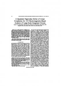
KD-trees are used to find the nearest point to a given point among a set of points in space. They operate by recursively partitioning a high-dimensional space by splitting it along one of its dimensions. Consider a three-dimensional space of points. At the top level, the space can be split along one of the axes. At subsequent levels, the sub-spaces can be similarly split along any axis. The basic operations of a kd-tree is to add and remove points and to issue the query nearest(a), which returns the nearest point to a. To illustrate these operations, we use a 1-dimensional kd-tree built over the points {2, 8, 11, 15, 25, 28, 30, 35}, shown in Figure 3(a). While there are many possible implementations of kd-trees, we describe the behavior of a tree implemented along the lines of the one used in [23], which is also used in the experiments presented in Section 7. Points are stored only in the leaf nodes of the kd-tree. Each interior node records the “pivot” point, which defines the split plane and is listed in the top half of the node. Each leaf node records a set of points contained in it, shown in the top half of the node. Both interior and leaf nodes maintain the range of all the points they contain, shown in the bottom half of the nodes. For each interior node, the pivot point is chosen to be roughly equidistant between the boundaries of the ranges of its leaves. Thus, the root node of the tree, node a, has subtrees containing the points {2, 8, 11, 15} and {25, 28, 30, 35} and has a pivot at 10. Given the kd-tree in Figure 3(a), we now describe how add, remove and nearest operate: • add: If we invoke add(16) on the kd-tree, the first step is to

determine which leaf node the point belongs to. We start at the root node and check the pivot point (in higher dimensions, the split plane) and find that we should check the left subtree. We recurse until we find the leaf node the point belongs to, in this case node e, and add it. Next, we check the ancestors of e to determine if the range field needs to be updated. The range of node b needs to be changed, as 16 lies outside its current range. The updated tree is shown in Figure 3(b). • remove: Removing a node is similar to adding a node. If we invoke remove(15) on the tree in Figure 3(b), we traverse the tree to find that 15 is in node e, and remove it. In this case, none of e’s ancestors need to be updated. The new tree is shown in Figure 3(c). • nearest: Invoking nearest(28) on the kd-tree in Figure 3(c) behaves as follows. First the same recursive search as used for add and remove is applied, and 28 is located in node f. Then, the nearest neighbor in the leaf node is found, in this case 25. Maintaining the current best match, the recursion is unwound to visit the parent of e, and the range of e’s sibling g is checked to see if any point could be closer to 25 than the current best match. Since the range 30–35 could contain a closer point, we visit g and find a new point that is a better match, 30. We then move up one level, reaching the root node. We again check the sibling tree, rooted at b, and find that no point in its range (2–16) could be closer to 28 than the current best match. This range check allows us to skip traversing that subtree. As we have reached the root node, the operation is complete and we return the current best match. 3

1 2 3 4 5 6 7 8 9 10 11 12 13 14 15 16 17 18 19 20 21 22 23 24 25 26 27 28 29 30 31 32

Graph g = / ∗ r e a d i n g r a p h ∗ / MST mst = new MST ( ) ; U n i o n F i n d u f = new U n i o n F i n d ( ) ; W o r k l i s t wl = new W o r k l i s t ( ) ; f o r e a c h ( Node n : g ) { uf . c r e a t e ( n ) ; wl . add ( n ) ; n . outEdges = n . getEdges ( ) ; } f o r e a c h ( Node n : wl ) { / / u n o r d e r e d a = u f . f i n d ( n ) ; / / f i n d r e p node f o r n Edge e = n u l l ; f o r ( Edge k : a . o u t E d g e s ) { Node p1 = k . g e t H e a d ( ) , p2 = k . g e t T a i l ( ) ; i f ( u f . f i n d ( p1 ) ! = a | | u f . f i n d ( p2 ) ! = a ) i f ( ( e ! = n u l l ) && ( k . w e i g h t ( ) < e . w e i g h t ( ) ) ) e = k; } i f ( e != n u l l ) { mst . add ( e ) ; / / add e d g e t o MST / / g e t r e p node f o r o t h e r e n d p o i n t b1 = u f . f i n d ( e . g e t H e a d ( ) ) ; b2 = u f . f i n d ( e . g e t T a i l ( ) ) ; i f ( b1 ! = a ) u f . u n i o n ( a , b1 ) ; / / merge c o m p o n e n t s else u f . u n i o n ( a , b2 ) ; c = u f . f i n d ( a ) ; / / f i n d new r e p node updateOutEdges ( c , a , b ) ; wl . add ( c ) ; } }

Figure 4. Pseudocode for Boruvka’s MST algorithm 2.3

Algorithms

Because we are interested in parallelism in programs, not merely data structures, it is important to consider how these data structures are used. In other words, the algorithm that manipulates the data structure is just as important to parallelism as the behavior of the data structure itself. We discuss the implications of this fact in Section 7. Kruskal’s Algorithm Union-find structures are used in Kruskal’s algorithm as discussed in Section 1. Boruvka’s algorithm The union-find data structure can be used when implementing Boruvka’s minimum spanning tree algorithm. The intuition behind Boruvka’s algorithm is that the MST starts as a forest, with each node in its own component. Each component then finds the lightest weight edge that connects it to another component, adds that edge to the MST and merges the two components together. The membership of nodes in components can be maintained using a union-find data structure, as shown in the pseudocode for Boruvka’s algorithm in Figure 4. The algorithm proceeds as follows. First, each node is placed into its own component, and has its outgoing edges recorded (lines 5–9). Next, the components are processed iteratively. Because the algorithm is unordered, this processing can happen in any order. For each component, the lightest edge connecting it to some other component is selected (lines 12–18). If the line is null, then this component is fully connected and has no more outgoing edges that can be placed in the MST. Otherwise, the edge is added to the MST (line 20), and the component is merged with the matching component (lines 22–23). We then find the representative node for the merged component (line 24), and update the outgoing edges by combining the outgoing edges of the two merged components (line 25). The new component is then added to the worklist (line 26). The algorithm terminates when all components have no more outgoing edges. In terms of amorphous data parallelism, the active nodes are the components in the worklist. The neighborhood of a 2009/10/5

a

a

20 2 — 35 b

c

10 2 — 15 d

e

2, 8 1—8

b

29 25 — 35 f

11, 15 11 — 15

d

30, 35 30 — 35

e

2, 8 1—8

20 2 — 35

c

10 2 — 16 g

25, 28 25 — 28

a

20 2 — 35 b

29 25 — 35 f

11, 15, 16 11 — 16

(a)

g

25, 28 25 — 28

c

10 2 — 16 d

30, 35 30 — 35

29 25 — 35

e

2, 8 1—8

f

11, 16 11 — 16

(b)

g

25, 28 25 — 28

30, 35 30 — 35

(c)

Figure 3. Different kd-tree states

1 2 3 4 5 6 7 8 9 10 11 12 13 14 15 16 17 18 19 20 21 22

KDTree k d t r e e = new KDTree ( p o i n t s ) ; Dendrogram dend = new Dendrogram ( ) ; W o r k l i s t wl = new W o r k l i s t ( ) ; foreach (p in points ) { wl . add ( p ) ; } f o r e a c h ( P o i n t p i n wl ) { / / u n o r d e r e d i f ( /∗ p i s c l u s t e r e d ∗/ ) continue ; P o i n t n = kdTree . n e a r e s t ( p ) ; i f ( n == p t A t I n f i n i t y ) break ; P o i n t m = kdTree . n e a r e s t ( n ) ; i f (m == p ) { C l u s t e r c = new C l u s t e r ( p , n ) ; k d T r e e . remove ( p ) ; k d T r e e . remove ( n ) ; k d T r e e . add ( c ) ; d e n d r o g r a m . add ( c ) ; wl . add ( c ) ; } else { wl . add ( p ) ; } }

=

(Obj + B + Z + null)

=

Possible abstract states of data structure

m∈M

=

Σ×V →Σ×V

i∈I

=

Z

τ ∈T

=

P(I)

Figure 6. Domains

be used to guarantee safe parallel execution. We will also use these definitions in subsequent sections to discuss the capabilities and limitations of various conflict detection mechanisms that have been proposed in the literature.

Figure 5. Pseudocode for unordered agglomerative clustering algorithm component includes its outgoing edges and whatever portions of the union find data structure are manipulated during the find and union operations. Agglomerative Clustering KD-Trees can be used in agglomerative clustering. The input to the algorithm is (1) a set of points, and (2) a metric which measures the distance between two points. The algorithm builds a hierarchical clustering of points, called a dendrogram, in a bottom-up manner, whose structure exposes the similarity between points. There are many different variants of agglomerative clustering, we evaluated the version described in [23]. The algorithm proceeds as follows. The kd-tree is built containing every point in space. A worklist is then initialized with every point. In each iteration, a point p is chosen from the worklist and its nearest neighbor n is found. We then find the nearest neighbor of n. If n’s nearest neighbor is p, then the two points are clustered and a new point is created. The kd-tree is updated, and the new point is added to the worklist. If n’s nearest neighbor is not p, then p is added back to the worklist to be processed later. The algorithm terminates when the worklist is empty. Pseudocode for this algorithm is shown in Figure 5. This algorithm is unordered, with the points remaining in the space representing the active nodes. The neighborhood is the portions of the kd-tree manipulated by each iteration.

3.

v∈V σ∈Σ

Formalizing Commutativity

In this section, we provide a precise definition of commutativity and commutativity conditions. We show how commutativity conditions, which are predicates on a data structure’s abstract state, can 4

3.1

State and Methods

We are concerned with amorphous data-parallel programs which manipulate data structures in parallel. A data structure is defined by its abstract state (e.g., for a set, the abstract state is the collection of elements it contains) and a set of methods that can be invoked on the data structure which manipulate that abstract state. We assume in this work that the data structure is linearizable [11]; colloquially, the method invocations on data structures are atomic. In the formalism we present, we assume that there is only one data structure in the system. The formalism easily extends to multiple data structures provided they have disjoint abstract state: invoking methods on one data structure cannot change the abstract state of another. We begin by formally defining a set of domains that will be used to discuss data structures, the methods they support, and their abstract state. These domains are shown in Figure 6. V ranges over integers, booleans, object references and null. Σ is the domain of abstract states of the data structure. We assume that the data structure also provides an operator, ≡Σ which determines if two abstract states are equivalent. M is the domain of methods. A method takes a data structure state and a value (our formalization assumes without loss of generality that methods take single arguments) and returns a new data structure state (to capture side effects) and a return value. Iterations are given unique labels in I. The set τ ∈ T tracks which iterations are active. Program states are represented by the tuple hσ, τi. We define a method invocation, mi (v), as a method m being invoked by a particular iteration i with an argument v. The denotation of a method invocation in a particular state maps program states to program states and a value (augmented with bottom): Σ × T → Σ × T × V⊥ 2009/10/5

In other words, invoking the methods in H in order produces the desired final state, and no method was invoked when its iteration was not active. We define the equivalence of two histories as follows:

and is defined as: Jmi (v)Kστ = hσ 0 , τ i, r⊥

where m(σ, v) = (σ 0 , r) r⊥ = r if i ∈ τ, ⊥ otherwise

Essentially, if iteration i executes method m with argument v in state σ, the new abstract state of the data structure is σ 0 , and the method returns r. If i is not an active iteration, we return ⊥ instead. We also define the following two special methods which maintain the set of active iterations: Jbegin(i)Kστ = hσ, τ 0 i, i where τ 0 = τ ∪ {i} Jend(i)Kστ = hσ, τ 0 i, i where τ 0 = τ /{i}

Note that in the following development, “method” refers to both methods invoked on the data structure as well as begin and end. We define two helper functions ps and ret that project out the program state and return value, respectively, from denotation of a method invocation. We can thus define sequential composition: Jα; βKστ , JβKps(JαKστ)

We define the equivalence of two program states in the natural way: D EFINITION 1. hσ, τi ≡ hσ 0 , τ 0 i

,

σ ≡Σ σ 0 ∧ τ = τ 0

In other words, two states are equivalent if they represent the same data structure state and the same iterations are active in both. L EMMA 1. If two program states are equivalent, applying the same method invocation to both will produce equivalent program states. ∀m, v, i . hσ1 , τ1 i ≡ hσ2 , τ2 i ⇔ Jmi (v)Kσ1 τ1 ≡ Jmi (v)Kσ2 τ2 P ROOF. Straightforward from definition of equivalence and method invocation semantics. 3.2

Histories and Serializability

In prior work ([9, 24]), parallel program executions are typically viewed as histories, with calls and responses to different methods interleaving into a sequential sequence of invocations. Because we assume that the data structure is linearizable, we need only express histories in terms of interleaved method invocations; methods are assumed to return immediately after they are invoked. A parallel execution history H consists of some initial program state hσ0 , τ0 i, a series of method invocations, mi0 (v0 ); mj1 (v1 ); ... , and a final program state, hσF , τF i. For brevity, we write M instead of mi (v) unless we need to refer to the iteration which invokes a method, or a method’s arguments. We can thus write histories as follows: H = M0 ; M1 ; M2 . Unless doing so is ambiguous, we will leave out the initial and final states when expressing histories. We will use the notation hσM ;H , τM ;H i to represent the intermediate state of a history H immediately before method invocation M (this is equivalent to the final state of a history H 0 where H 0 has the same initial state as H and consists of the prefix of H up to invocation M ). We now define various common terms such as “validity” and “serializability” in terms of our formalism. D EFINITION 2. A history H with final state hσF , τF i and initial state hσ0 , τ0 i is VALID if the sequential composition of its method invocations, starting from hσ0 , τ0 i results in hσF , τF i, and: ∀M ∈ H . ret(JM KσM ;H τM ;H ) 6= ⊥ 5

D EFINITION 3. For histories H1 and H2 with final states hσ1 , τ1 i and hσ2 , τ2 i, respectively, we define H1 to be equivalent to H2 (written H1 ≡ H2 ) if and only if both are valid and there exists a one-to-one mapping, η, between method invocations in H1 and method invocations in H2 such that: hσ1 , τ1 i ≡ hσ2 , τ2 i ∧ ∀M1 ∈ H1 , M2 = η(M1 ) . ret(JM1 KσM1 ;H1 τM1 ;H1 ) = ret(JM2 KσM2 ;H2 τM2 ;H2 )

In other words, two histories are the same if and only if they produce the same final state, they contain the same methods (in some order), and every method returns the same value. In prior work, such as [9], two histories are defined to be equivalent if, when they are extended by other histories, their extensions are equal. Unlike such earlier definitions of equivalence, our definition allows for “local” determination of equivalence where we need not reason about future method invocations. We next define the well-known notion of serializability [1] in terms of our formalism. D EFINITION 4. A history H with final state hσ, τi is SERIALIZED with respect to its initial state hσ0 , τ0 i if it is VALID, and for any two invocations M1 and M2 in H made by the same iteration i, there is no intervening invocation M3 made by iteration j where j 6= i. D EFINITION 5. A history H is SERIALIZABLE iff there exists a 0 0 SERIALIZED history H such that H ≡ H . Because of our definition of history equivalence, this definition of serializability is analogous to the notion of view serializability in databases [1], where all reads (i.e., return values of method invocations) return the same values. Note that we require that the final data structure states of the two histories be equivalent. We can now define the semantics of an unordered amorphous data parallel iterator by appealing to the history produced by its parallel execution. D EFINITION 6. Let state hσ0 , τ0 i represent the state of an amorphous data-parallel program immediately before parallel execution of an unordered iterator begins. Let H represent the history of parallel execution. The program’s parallel execution matches its sequential semantics if every active element is processed2 and if H is SERIALIZABLE. This satisfies the semantics of amorphous data parallelism because unordered amorphous data-parallel iterators can process iterations in any order. A similar definition can be given for ordered iterators, provided that the definition of SERIALIZABLE is modified to only allow sequential orders of iterations that obey the ordering constraints of the ordered iterator. 3.3

Commutativity

In this subsection, we present a precise definition of commutativity conditions, which specify the conditions under which two method invocations commute. We begin by defining commutativity for a pair of method invocations: 2 In

this paper we do not formally define what “every active element is processed” means, but informally it means that every active element that is generated during the execution of the program is processed to completion by exactly one iteration. In general, we will assume that there is an external scheduling mechanism which ensures this.

2009/10/5

D EFINITION 7.

COMMUTES(M1 , M2 , hσ, τi)

:

history is C - VALID if:

ps(JM1 ; M2 Kστ) ≡ ps(JM2 ; M1 Kστ) ∧ ret(JM1 ; M2 Kστ) = ret(JM2 Kστ) ∧

∀mip (vp ) ∈ H . ∀mjq (vq ) ∈ A(mip (vp )) . φmq ;mp is C - INVARIANT and

ret(JM2 ; M1 Kστ) = ret(JM1 Kστ) ∧

φmq ;mp (vq , vp , hσmq , τmq i, hσmp , τmp i)

Intuitively, two method invocations commute starting from a given state if and only if invoking them in either order produces equivalent states and the return values of both invocations are the same regardless of their order. The special functions begin and end commute with all methods invoked by other iterations, but not with methods invoked by the same iteration. Unlike previous work, we define commutativity in terms of a specific state rather than all states. For our purposes, we are concerned with whether one history can be transformed into another by swapping commuting invocations: D EFINITION 8. Two histories H and H 0 are C - EQUIVALENT (H ≡C H 0 ) if H can be transformed into H 0 by a sequence of swaps of pairs of consecutive, commuting method invocations. Note that H ≡C H 0 ⇒ H ≡ H 0 , but not vice-versa. Finally, we define commutativity conditions: D EFINITION 9. The commutativity condition, φm1 ;m2 for a pair of methods m1 and m2 is a predicate with signature: V ×V ×Σ×T ×Σ×T →B such that: φm1 ;m2 (v1 , v2 , hσ, τi, hσ 0 , τ 0 i) ⇒ ∀i, j . COMMUTES(mi1 (v1 ), mj2 (v2 ), hσ, τi) Hence, a commutativity condition is a predicate which evaluates to true only if two methods commute in a particular state. Note that these conditions can be dependent on the two states in which the methods are executed, although the methods only commute in one state. We further refine commutativity conditions by defining: D EFINITION 10. A predicate which is a function of state, p(hσ, τi) is C - INVARIANT if and only if: ∀H, H 0 , H ≡C H 0 . ∀M ∈ H . p(hσM ;H , τM ;H i) ⇔ p(hσM ;H 0 , τM ;H 0 i) Informally, given a history H, a predicate dependent on state that holds immediately before a method is executed always holds immediately before the method is executed, even if commuting methods are swapped. In other words, if a C - INVARIANT predicate holds before a method in one history, it holds before that method in all C - EQUIVALENT histories. Note that if a commutativity condition does not refer to program state, it is trivially C - INVARIANT. 3.4

Using commutativity to prove serializability

Let us define active methods: D EFINITION 11. A method mi1 invoked by iteration i is ACTIVE with respect to another method mj2 invoked by iteration j in a history H iff: (i) i 6= j; (ii) mi1 appears before mj2 in H; and (iii) end(i) appears after mj2 in the H. In other words, a method invocation is active with respect to another if it was invoked earlier and the iteration that invoked it is still in the active set when the second method is invoked. D EFINITION 12. Let A(mik (v)) be the set of all method invocations that are ACTIVE with respect to a method invocation in H. A 6

(1)

In other words, a history is C - VALID if every method invocation in the history commutes with every method invocation that was ACTIVE when it was invoked. We can now prove the following theorem. T HEOREM 1. Let H be a valid history of the parallel execution of an amorphous data-parallel program. If H is C - VALID, then H is SERIALIZABLE and the serialized history is C - EQUIVALENT to H. P ROOF. The proof proceeds by induction on the length of histories. We will proceed by assuming there are only two iterations in the history, and neither has ended. We will generalize at the end of the proof. The base case is when there are only two invocations in the history: Base case: H = mi0 (·); mj0 (·) or H = mj0 (·); mi0 (·). H itself is SERIALIZED

Inductive hypothesis: If H has length k it is serializable and the serialized equivalent is C - EQUIVALENT to H. Show: H with length k + 1 is serializable. Define H− such that H = H− ; Mk+1 , where H− has length k. By the inductive hypothesis, there is another history H 0 of length k which is C - EQUIVALENT to H− and SERIALIZED. By the definition of SERIALIZED, assume without loss of generality H 0 = Hi ; Hj where Hi consists of only invocations by iteration i, and Hj contains only invocations by j. We now have two cases: • Case 1: Mk+1 was invoked by iteration j.

Obviously, Hi ; Hj ; Mk+1 is SERIALIZED. By Lemma 1, Hi ; Hj ; Mk+1 ≡ H− ; Mk+1 , therefore H ≡C Hi ; Hj ; Mk+1 . • Case 2: Mk+1 was invoked by iteration i. We note that every invocation made by j in Hj is ACTIVE with respect to Mk+1 . By Equation (1), we know that Mk+1 commutes with all invocations made by j in H− . Because the commutativity conditions are C - INVARIANT, we have that Mk+1 commutes with all invocations made by j in Hi ; Hj . By the definition of commutativity, we can easily show (through induction on the length of Hj ) that Hi ; Hj ; Mk+1 ≡C Hi ; Mk+1 ; Hj . The latter history is SERIALIZED. By Lemma 1, we see that H ≡C Hi ; Mk+1 ; Hj . Because in both cases, H is C - EQUIVALENT to a SERIALIZED history, we have shown that H is serializable and its serialized equivalent is C - EQUIVALENT to H. We now generalize from the initial assumption in two ways. First, we consider the effect of more than two iterations. This is handled in a straightforward manner. According to Equation (1) each method is checked for commutativity against active methods from every iteration. Thus, the proof techniques which applied for two iterations can be extended: methods which were previously “pushed” back across methods from one iteration in Case 2 above will now be pushed back across methods from multiple iterations. The second generalization is to consider histories when some iterations have invoked end. Consider a history H with three iterations i, j, k where i and j are active throughout and k ends in the middle. Let Hk be a history with i, j, k active throughout such that H = Hk ; Hij where only i and j invoke methods in Hij . We can now apply the multi-iteration version of the proof to Hk to show that it is C - EQUIVALENT to a serialized history with all invocations 2009/10/5

2. Derive the state hσmk , τmk i in which mk was executed by executing the inverses of all subsequent methods in H. 3. Evaluate φmk ;mi (vk , v, σmk , τmk , σc , τc ) 4. If φ is false: (i) roll back either iteration i or the iteration which executed mk by invoking inverse actions; (ii) execute end(·) for whichever iteration rolled back; and (iii) if i was rolled back, stop processing the current method. 5. Restore hσc , τc i by re-executing forward methods.

by k at the beginning: Hk+ ; Hk− where Hk+ contains only invocations from k and Hk− contains only invocations by i and j (and is serialized). Thus, H ≡C Hk+ ; Hk− ; Hij . Because H is C - VALID , all the methods in Hij commute with all the methods in Hk− (because the φs are C - INVARIANT), and so by induction on the lengths of Hk− and Hij , we can show that H is serializable. Note the methods in Hk+ are inactive with respect to the methods of Hij and we do not need to appeal to their commutativity. Crucially, Theorem 1 implies that to show that a parallel execution history of an amorphous data parallel program using an unordered iterator satisfies the sequential semantics, we need only show that the history is C - VALID. This theorem motivates a system that can guarantee correct parallel execution, which we present in Section 3.6. As an aside, showing that a schedule is view-serializable is NP complete, so showing that a history H has an equivalent serialized schedule is also NP -complete. However, Theorem 1 provides sufficient conditions under which H is serializable, not necessary ones. Specifically, Theorem 1 guarantees a form of serializability that is a generalization of d-serializability [18]. A history is d-serializable if non-interfering operations can be swapped to produce a serial schedule. The definition of non-interference in [18] can be generalized to encompass commuting methods. 3.5

Inverse Methods

To complete the formal specification of commutativity, we introduce the notion of inverse methods: D EFINITION 13. A method qm ∈ M is an m iff

INVERSE

of a method

∀hσ, τi, i, v . ∃v 0 . i as(Jmi (v); qm (v 0 )Kστ) ≡ σ ∧

This conflict detection scheme clearly ensures that the history remains C - VALID, and hence SERIALIZABLE, throughout parallel execution. This approach ensures that the parallel execution of an amorphous data-parallel program respects its sequential semantics, provided another mechanism ensures that any active elements being processed by iterations that roll back get processed eventually. Unfortunately, this baseline conflict detection scheme is very inefficient, as it requires rollbacks and re-execution to verify commutativity. In the next section, we provide a number of example commutativity conditions and define a number of properties of commutativity conditions. In Sections 5 and 6, we will present other more efficient conflict detection approaches and discuss the properties commutativity conditions must possess for those approaches to be applied effectively.

4.

Commutativity Conditions

In this section, we will describe the commutativity conditions for a number of data structures, including the “challenge” data structures described in Section 2. We will then define two properties of commutativity conditions: ONLINE - CHECKABLE and SIMPLE. Sections 5 and 6 will discuss how these properties influence the applicability of various conflict detection mechanisms. 4.1

∀hσ 0 , τ 0 i, m∗ , v∗ , j, k . j

COMMUTES(m

(v), mk∗ (v∗ ), hσ 0 , τ 0 i)

Commutativity Conditions

When writing commutativity conditions, we use the notation

⇔

m1 (a)/rσ commutes with m2 (b)/rσ0 if ψ

j 0 k 0 0 COMMUTES(qm (v ), m∗ (v∗ ), hσ , τ i)

to describe φm1 ;m2 , which is shorthand for:

where as projects out data structure state. Informally, an inverse method reverses the effects of its associated forward method, and an inverse method commutes with everything its forward method commutes with. We can thus show: T HEOREM 2. If a C - VALID history H has the form H1 ; m; H2 , and we invoke qm where qm is the inverse of m, H1 ; m; H2 ; qm is C VALID and produces the same abstract state as H1 ; H2 . P ROOF. Follows from the definitions of C - VALID and INVERSE and induction on the length of H2 . This means that by invoking an inverse method at any time in a C VALID history, we leave the data structure in the same state as if the forward method had never occurred. 3.6

6. If all φs are true, execute mi and continue.

Conflict detection using commutativity conditions

We can exploit Theorems 1 and 2 to define a baseline conflict detection mechanism. Intuitively, the mechanism tracks method invocations on a data structure as they happen. The scheme is initialized with state of the system before parallel execution, and an empty history, H. Then, every time it sees a method mi (v) invoked by iteration i on the data structure, it performs the following steps: 1. Determine which methods are ACTIVE. 2. Verify that H; mi is C - VALID. For each active method mk (vk ): 1. Let the current state be hσc , τc i. 7

φm1 ;m2 (a, b, hσ, τi, hσ 0 , τ 0 i) = let rσ = retJm1 (a)Kστ in let rσ0 = retJm2 (b)Kσ 0 τ 0 in ψ Note that when φ is evaluated for two particular method invocations, as in Theorem 1 or in the baseline conflict detection scheme, the states used are the states in which the methods were actually invoked. For brevity, we drop the “if ψ” portion of the condition if the condition is always true. Unless otherwise specified, the commutativity conditions we provide are symmetric. An interesting point about these commutativity conditions is that they are only dependent on the abstract state of a data structure, not its concrete state. Thus, commutativity conditions that are valid for, e.g., one implementation of a set are valid for all set implementations. Crucially, this means we need only determine a commutativity specification once for each type of abstract data structure (sets, maps, graphs, etc.), rather than anew for each data structure implementation. We now present the commutativity specifications for a number of data structures. While the conditions we show are correct (according to definition 9) and C - INVARIANT, formally proving either proposition is beyond the scope of this paper. Accumulator An accumulator is a counter which supports two methods, increment and read with the obvious semantics. The commutativity conditions are given in Figure 7. Condition (1) 2009/10/5

(1) (2)

increment(a) increment(a)

(3)

read()/rσ

commutes with commutes with if commutes with

Definitions:

increment(b) read()/rσ0 false read()/rσ0

repσ (x) = ret(Jfind(x)Kστ) rank(x) = the “rank” of x (as defined in union-by-rank).  repσ (x) if rank(repσ (x)) < rank(repσ (y)) loserσ (x, y) = repσ (y) otherwise

Figure 7. Commutativity conditions for accumulator data structure. (1)

add(a)/rσ

(2)

add(a)/rσ

(3)

add(a)/rσ

(4)

remove(a)/rσ

(5)

remove(a)/rσ

(6)

remove(a)/rσ

commutes with if or commutes with if commutes with if commutes with if or commutes with if commutes with

add(b)/rσ0 a 6= b rσ = false ∧ rσ0 = false remove(b)/rσ0 a 6= b contains(b)/rσ0 a 6= b ∨ rσ = false remove(b)/rσ0 a 6= b rσ = false ∧ rσ0 = false contains(b)/rσ0 a 6= b ∨ rσ = false contains(b)/rσ0

(1)

union(a, b)

(2)

union(a, b)

(3)

union(a, b)

(4) (5)

find(a)/rσ find(a)/rσ

(6)

create(a)/rσ

commutes with if and commutes with if commutes with if commutes with commutes with if commutes with if

union(c, d) repσ (c) 6= loserσ (a, b) repσ (d) 6= loserσ (a, b) find(c)/rσ0 repσ (c) 6= loserσ (a, b) create(c)/rσ0 false find(b)/rσ0 create(b)/rσ0 false create(b)/rσ false

Figure 10. Commutativity conditions for union-find data structure.

Figure 8. Commutativity conditions for set data structure. Definitions: dist(a, b) is an algorithm defined-distance metric such that nearest(a) returns the nearest point according to dist. (1) (2)

nearest(a)/rσ nearest(a)/rσ

(3)

nearest(a)/rσ

(4)

remove(a)/rσ

(5)

remove(a)/rσ

(6)

add(a)/rσ

commutes with commutes with if or commutes with if or commutes with if or commutes with if commutes with if or

nearest(b)/rσ0 add(b)/rσ0 rσ0 = false dist(a, b) > dist(a, rσ ) remove(b)/rσ0 a 6= b ∧ rσ 6= b rσ0 = false remove(b)/rσ0 a 6= b rσ = false ∧ rσ0 = false add(b)/rσ0 a 6= b add(b)/rσ0 a 6= b rσ = false ∧ rσ0 = false

(3), (5) and (6) state that create does not commute with anything— new sets can only be created while no other iteration is accessing the data structure. As expected, find operations commute with each other (condition (4)). Most complex are the conditions dealing with union. We define two helper functions: repσ (a) which returns a’s representative node in state σ; and loserσ (a, b) which finds the representative nodes of a and b in state σ and returns the one with lowest rank or repσ (b) if the ranks are equal. Condition (1) states that two unions commute as long as the second doesn’t operate on the loser from the first. Note that this is defined by evaluating rep on the arguments to the second union in the state that the first union executed in. Similarly, condition (4) states union commutes with find provided that find would not have returned the loser of the union had it been executed in σ. 4.2

Figure 9. Commutativity conditions for kd-tree data structure. states that increments commute with each other, and condition (3) states that reads commute with each other. Condition (2) states that increment never commutes with read. Set A set provides three methods: add, read and contains where add and remove return true if they modified the set, and false otherwise. The commutativity conditions for sets are in Figure 8 and are largely straightforward. Methods commute with each other if (i) neither modifies state (as in the case of contains or add/remove calls that return false) or (ii) their arguments are different. KD-Tree A kd-tree supports the methods as defined in Section 2.2. The commutativity conditions for kd-trees are given in Figure 9. The commutativity conditions (4–6), are similar to those for sets. The conditions dealing with nearest however, are more complex. Recall that the nearest(a) returns the point closest to a according to a distance metric dist. As nearest is a read-only operation, it clearly commutes with itself, as stated in condition (1). Condition (3) states that nearest commutes with remove as long as remove does not remove either the argument or return value of nearest. Condition (4) states that nearest(a) commutes with add(b) as long as add(b) does not modify state, or b is not closer to the a than the return value of nearest(a) is. Union-find The union-find data structure, defined as in Section 2.1 has the most complex commutativity conditions. Conditions 8

Properties of Commutativity Conditions

An interesting property that some commutativity conditions have is ONLINE - CHECKABILITY , which we define negatively for comprehensibility: D EFINITION 14. φm1 ;m2 (v1 , v2 , hσ1 , τ1 i, hσ2 , τ2 i) is not ONLINE CHECKABLE if and only if φm1 ;m2 contains a clause which requires invoking some method m∗ (v∗ ) on state hσ1 , τ1 i and v∗ is dependent on m2 (·), v2 or hσ2 , τ2 i (including the result of invoking m2 (v2 ) in hσ2 , τ2 i). In other words, if a commutativity condition requires invoking a method on hσ1 , τ1 i using information that is related to hσ2 , τ2 i, the condition is not ONLINE - CHECKABLE. The nomenclature is inspired by the baseline conflict detection algorithm presented in Section 3.6. If a condition φm1 ;m2 is ONLINE - CHECKABLE , there are no clauses which require knowing what m2 or its arguments are when invoking methods on hσ1 , τ1 i. Hence the predicate can be evaluated without rolling back state. Any clauses dependent on hσ1 , τ1 i can be evaluated and recorded when m1 is invoked on hσ1 , τ1 i, and any clauses dependent on m2 , v2 or hσ2 , τ2 i can be evaluated when m2 is invoked on hσ2 , τ2 i. At that point φm1 ;m2 can be fully evaluated. We will take advantage of this property in Section 6. The commutativity conditions given for accumulators, sets and kd-trees are all ONLINE - CHECKABLE. Although condition (2) for the kd-tree requires evaluating dist, the method is not dependent on state, and so can be checked when m2 is invoked. Conversely, conditions (1) and (2) for the union-find data structure require invoking rep in the state of the first method invocation, but with the argu2009/10/5

ments of the second method invocation. Hence, conditions (1) and (2) for the union-find data structure are not ONLINE - CHECKABLE. Next, we define an even more restrictive property of commutativity conditions, called SIMPLE: D EFINITION 15. A commutativity condition φm1 ;m2 is SIMPLE if it is a conjunction of clauses of the form a 6= b where every a is an argument or return value of m1 and every b is an argument or return value of m2 . The commutativity conditions for accumulators are SIMPLE, as are conditions (2) and (6) for sets, conditions (1) and (5) for kdtrees and conditions (3–6) for union find structures. We will take advantage of this property in Section 5.2.

5.

Approaches to conflict detection

In this section, we discuss two prior approaches to detecting conflicting concurrent accesses to shared data structures. First is memory level locks, where locks are placed on concrete memory locations or objects, and second is abstract locks, where locks are placed on abstract pieces of data, rather than concrete locations. We discuss how these techniques can be used to express commutativity conditions, and when they cannot capture the concurrency allowed by a commutativity specification. For abstract locking, we also provide a construction by which an abstract locking scheme can provide conflict detection for a data structure that fully captures commutativity. To describe the expressivity of conflict detection, we introduce the notion of a conflict detection scheme’s compatibility with a commutativity specification: D EFINITION 16. A conflict detection scheme is COMPATIBLE with a commutativity specification for a data structure if the invocation of two methods m1 and m2 by different iterations on that data structure are permitted to proceed concurrently by the conflict detection mechanism if and only if m1 and m2 commute according to the commutativity specification. The baseline conflict detection scheme presented in Section 3.6 is COMPATIBLE with a data structure’s commutativity conditions by construction. 5.1

Memory-level Locks

Memory-level locking refers to any locking strategy where locks are placed on all the concrete memory locations accessed by a thread while processing an active element in an amorphous dataparallel program. In other words, when a thread invokes methods on a data structure, it acquires either shared locks (in the case of reads) or exclusive locks (in the case of writes) on every memory location it touches. Alternately memory-level locking can be formulated in terms of locks on concrete objects in the heap, rather than individual memory locations. Conceptually, memory-level locking captures the following execution strategy: every memory location or concrete object accessed while processing an active element is placed in its neighborhood; two active elements can be processed in parallel if their neighborhoods only overlap in regions where both elements read data. In the abstract, memory level locking is the strategy employed by parallelization schemes based on either transactional memory (TM) [3] or thread-level speculation (TLS) [19, 12]. While both thread-level speculation and transactional memory have numerous implementations, they fundamentally rely on locking either memory locations, as in TLS and hardware implementations of TM [8, 16], or every concrete object accessed during parallel execution, as in many software implementations of TM [10, 20]. Memory-level locking is often not compatible with commutativity. This is because data structures often maintain significant 9

amounts of metadata, which is used to improve performance but carries no semantic content (e.g., the range information maintained by the kd-tree). Union-find data structures make use of parent pointers and path compression to accelerate find operations, as discussed in Section 1. Unfortunately, memory-level locking requires tracking accesses to metadata as well as the data in a structure; performing path compression during a find operation places all the updated parent pointers in an active element’s neighborhood. As a result, even though commutativity allows two find operations on the same set to proceed concurrently, memory level locking will necessarily result in a conflict, as the two neighborhoods will overlap. An interesting question is, when is memory-level locking compatible with commutativity? Because memory-level locking places locks on metadata, and this metadata is not part of the semantic specification of commutativity, trouble arises when two methods which semantically commute (in other words, they access disjoint regions of a data structure’s semantic state) nevertheless access the same metadata in a conflicting manner. T HEOREM 3. Memory level locking for a particular data structure implementation is compatible with a commutativity specification if and only if, for all pairs of methods m1 and m2 , φm1 ;m2 implies that m1 and m2 either access disjoint data and metadata or any data and metadata accessed by both methods is only read. P ROOF. This is straightforward from the semantics of memorylevel locking and the definition of compatibility. Note that the compatibility of memory level locking depends not only on the commutativity specification (i.e. a data structure’s abstract state) but also its implementation (i.e. a data structure’s concrete state). Trivial examples of data structures which are compatible with memory-level locking are those which do not maintain metadata, such as dense matrices and arrays. 5.2

Abstract Locks

Because memory-level locking mechanisms limit parallelism when accessing data structures with a lot of metadata, there have been several proposals to use higher-level, abstract locks rather than locks on concrete memory locations and objects [17, 9]. Rather than locking every location accessed during a method invocation, abstract locking approaches only lock the relevant semantic data, but not the metadata. As such, when an active element is processed and a method is invoked on a data structure, only the relevant data is added to the element’s neighborhood, not any metadata. Note that because the metadata is not protected by the conflict detection scheme, other approaches must be taken to ensure that the data structure remains in a consistent state. Abstract locking is wellsuited to providing conflict checking for collections [4, 17] and other basic data structures [9]. However, it turns out there are more complex data structures, such as union-find structures and kd-trees, where abstract locking is insufficient to capture all the parallelism allowed by the commutativity conditions we presented in Section 4.1. To see why this is so, we must first define what abstract locking mechanisms provide. Unfortunately, to our knowledge no prior work formalizes how abstract locks work and what their capabilities are. To this end, we first define abstract locks and then describe how abstract locks can be used to implement conflict detection schemes. D EFINITION 17. An ABSTRACT LOCK is a lock consisting of a number of modes. When attempting to acquire a lock in a particular mode, the acquisition succeeds if no other entity holds the lock in 2009/10/5

an incompatible mode. The compatibility of modes is determined by a lock’s compatibility matrix. Note that abstract locks according to this definition are a generalization of database mode locks [7] and subsume the abstract locks used in [17]. These locks support a number of locking paradigms. For example, a traditional mutual exclusion lock is an abstract lock with one mode that is incompatible with itself. A reader-writer lock has two modes, where the reader mode is compatible with itself (allowing multiple readers) but incompatible with write mode, while the write mode is incompatible with all modes (allowing but a single writer). A generic abstract locking scheme for a data structure operates as follows: the data structure associates an abstract lock with each of its data members (defined as any arguments or return values to methods of the data structure). The data structure also has an abstract lock which represents whole data structure. When a method is invoked, the abstract locks on its arguments and on the data structure may be acquired in some mode, and when the method returns, the abstract lock on the return value may be acquired in some mode. This generic locking scheme can be instantiated by choosing which locks are acquired, and in which modes, and the particular mode compatibility matrix for the abstract lock. This leads to the following definition: D EFINITION 18. An abstract locking scheme is PROPER if it is an instantiation of the generic abstract locking scheme. The abstract locking schemes presented in prior work on abstract locking ([4, 9, 17]) all satisfy Definition 18. They also satisfy the following definition: D EFINITION PROPER and

19. An abstract locking scheme is VALID if it is the scheme only allows methods to proceed in parallel if they commute according to the data structure’s commutativity specification. A given data structure may have multiple valid abstract locking schemes. Consider, for example, the set data structure from Figure 8. One potential scheme is to acquire an exclusive lock on every element that is passed as an argument to add, remove and contains. It is apparent that this scheme is valid, as it only allows concurrent invocations to methods that commute. However, this scheme is not COMPATIBLE (according to Definition 16) with the set’s commutativity specification; concurrent calls to contains(x) will be disallowed, even though they commute. An alternate locking scheme— used in [9]—is to use read/write locks and acquire locks in write mode when calling add and remove, and in read mode when calling contains. Interestingly, even this scheme is incompatible with the commutativity specification: concurrent calls to add(x) that return false are prohibited, even though they commute. Not all data structures can support compatible, valid abstract locking schemes. For example, the kd-tree example in Figure 9 relies on evaluating a function (to find the distance between two points) to determine whether nearest commutes with add. This type of complex condition cannot be captured by abstract locks as defined by Definition 17. Similarly, the union-find data structure of Figure 10 requires determining the “loser” of a union to ensure commutativity; this information is not available to a proper abstract locking scheme, as defined in Definition 18. In Section 6, we describe how commutativity conditions for such structures can be implemented.

inc:ds inc:x read:ds read:ret

inc:ds √ √ × √

inc:x √ √ √ √

read:ds × √ √ √

read:ret √ √ √ √

(a) Compatibility matrix for accumulator abstract locks inc:ds read:ds

inc:ds √ ×

read:ds × √

(b) Reduced compatibility matrix

Figure 11. Compatibility matrices for accumulator abstract locks tions under which a compatible abstract locking scheme can be constructed. We can show: T HEOREM 4. Given a commutativity specification for a data structure, if for all commutativity conditions φm1 ;m2 one of three conditions holds: (i) φm1 ;m2 = false (i.e. the two methods always conflict); (ii) φm1 ;m2 = true (i.e., the two methods always commute) or (iii) φm1 ;m2 is SIMPLE, then a compatible, valid abstract locking scheme exists for the data structure. P ROOF. The proof proceeds by construction. We present the construction using the accumulator example from Figure 7. Recall that, by the generic abstract locking scheme, an abstract lock is associated with each data entity and with the data structure itself. Each lock supports a number of modes: each method requires one mode to represent its access to the data structure as a whole, and one mode for each argument and return value of the method. Thus, the locks used in the accumulator support four modes: increment(x) uses two modes, one for its argument (called inc:x) and one for the data structure (called inc:ds); read()/rσ uses two modes, one for its return value (called read:ret) and one for the data structure (called read:ds). Any time a method is invoked it acquires the data structure lock in its mode, as well as locks on all its arguments in their appropriate modes. For example, increment acquires the data structure lock in inc:ds mode, and lock on its argument in inc:x mode. Next, we determine in the compatibility matrix between the various modes, by considering each pair of methods m1 and m2 and their conflict conditions, and applying the following three rules to determine which locks must be acquired and the compatibility matrix for the locks: 1. If φm1 ,m2 = false, the two data structure modes are incompatible, but all other modes are left undefined. Hence, inc:ds is incompatible with read:ds. 2. For each conjunct x 6= y in φm1 ,m2 , where x is an argument or return value of m1 and y is an argument or return value of m2 , we set modes m1 :x to be incompatible with mode m2 :y. 3. Any pair of lock modes whose compatibility is left undefined by rules 1 and 2 are assumed to be compatible. The compatibility matrix thus generated for the accumulator is as shown in Figure 11(a). It is straightforward to verify that abstract locking schemes constructed by this approach are valid and compatible.

Because there are many possible valid abstract locking schemes for a given data structure, we would like to find sufficient condi-

Given the full compatibility matrix, we note that if a lock mode is compatible with all other lock modes, acquiring it is superfluous. Thus, we can eliminate any such lock modes, and remove the corresponding lock acquisitions from the relevant methods. This optimization yields the reduced compatibility matrix in Figure 11(b). The final abstract locking scheme acquires the data structure lock in inc:ds mode whenever increment is called, allowing other calls to increment to proceed, and read equivalently acquires the lock in

10

2009/10/5

5.2.1

Building compatible abstract locking schemes

read:ds mode. Note that this abstract locking scheme required general abstract locks; if abstract locks were restricted to read/write locks, the compatibility matrix in Figure 11(b) would be inexpressible.

6.

Gatekeeping

In this section, we present a new conflict detection paradigm called gatekeeping. A gatekeeper is a special object associated with a particular data structure whose role is to ensure that methods invoked by concurrently executing iterations on a data structure respect the specified commutativity conditions. At a high level, gatekeepers operate as follows. When an iteration i invokes a method m on a data structure, the gatekeeper “intercepts” the invocation and determines if the method invocation commutes with all other active method invocations (i.e., methods invoked by all iterations i for which end(i) has not yet been invoked). If the invocation commutes with all active method invocations, it is allowed to proceed and the iteration receives the result. If the invocation does not commute, then the gatekeeper invokes an arbitration mechanism which either rolls back i or the iteration j which invoked the method that m does not commute with. When determining if a method m1 commutes with an active method m2 , the gatekeeper is allowed to evaluate predicates on the arguments and return values of m1 and m2 . Additionally, the gatekeeper can invoke methods on the data structure it protects. The ability to evaluate arbitrary predicates and methods makes the gatekeeping approach strictly more expressive than abstract locking. Note that because a gatekeeper interacts with a data structure only by invoking methods on it, the data structure is effectively a “black box.” This means that the gatekeeper is agnostic to the actual implementation details of the data structure, and a gatekeeper constructed to protect one abstract data type (e.g., a gatekeeper which protects sets) can protect all implementations of that abstract data type. The gatekeeper deals with multiple concurrently executing iterations. To correct operation, the behavior of the gatekeeper itself must appear atomic. In other words, the entire sequence of events: (i) intercepting a method invocation, (ii) checking commutativity; (iii) executing the method on the data structure, and (iv) returning the result to the invoking iteration, should appear atomic. The overall data structure, including gatekeeping, should remain linearizable. There are two types of gate-keepers. The first type, forward gatekeepers, can only implement commutativity conditions which are ONLINE - CHECKABLE (see Definition 14), while the second, general gatekeepers, can implement any commutativity conditions that are C - INVARIANT (see Definition 10). We describe how each type operates and provide examples of how forward gatekeepers can protect kd-trees and general gatekeepers can protect union-find structures. 6.1

Forward gatekeepers

As an example of the procedure outlined above, we can define a forward gatekeeper for kd-trees. Whenever nearest(x) is invoked, the gatekeeper stores the tuple hx, dist(x, nx )i in a set. When add(b) is invoked, the gatekeeper iterates through the set, and for each tuple ha, dist(a, na )i evaluates dist(a, b) > dist(a, na ) to determine if the invocations of add(b) and nearest(a) commute. Similar techniques can be used to determine the commutativity of other methods. Crucially, the gatekeeper can determine commutativity simply by recording information about method invocations as they happen, rather than well after they execute. 6.2

General gatekeepers

General gatekeepers are conflict detection schemes that can capture any set of C - INVARIANT commutativity conditions. For conditions which are not ONLINE - CHECKABLE, the gatekeeper will perform an appropriate series of undo actions to bring the data structure to a state where the conditions can be evaluated, and then perform the necessary forward actions to restore the data structure state. This means that the gatekeeper must keep a log of all actions in case they need to be rolled back to check commutativity. Note that this entire process must appear atomic. General gatekeepers are a concrete implementation of the baseline conflict detection scheme presented in Section 3.6. 6.2.1

A general gatekeeper for union-find

We now describe the design of a general gatekeeper that fully captures the commutativity conditions of Figure 10 for the operations union and find. The union-find gatekeeper maintains two logs: findreps which stores all the active elements that have been returned by a call to find as representatives of some set, and loser-rep, which records the result of evaluating loser(a, b) whenever union(a, b) is invoked. For each invocation, union(a, b), the gatekeeper first computes loser(a, b). If the loser has been recorded in the find-reps log as the return value of an active find, then a conflict is detected. Additionally, if either of these representatives has been recorded in the loser-rep log as the loser representative involved in a previous union, then a conflict is detected. The gatekeeper subsequently performs the call to union, and updates loser-rep appropriately. In the case of an invocation find(a), the gatekeeper first executes the actual call on the data structure, getting the result ra . A subtle, but important point is that if find(a) had executed earlier, before some active invocation of union, it may have returned a different result. This is captured in condition (2) of Figure 10 as commutativity dependent on the results of calling find in a different state. To ensure that commutativity holds, the gatekeeper undoes the effects of all potentially interfering calls to union, and re-executes find(a) to ensure it still returns ra . If so, invoking find(a) does not violate commutativity. If not, a conflict is detected. The gatekeeper then restores the state of the data structure by re-invoking the unions. Finally, the ra is stored in find-reps to aid in conflict checking.

At an abstract level, forward gatekeepers operate as follows. Each method m has associated with it a set Cm of clauses. Each commutativity condition φm1 ;m2 is split into clauses that are dependent on the state in which m1 is executed and clauses that are dependent on the state in which m2 is executed. The former clauses are added to the set of clauses associated with m1 , Cm1 . Whenever a gatekeeper sees a method invocation, m(v), it evaluates every clause in Cm and records the results of evaluating those clauses, and the return value of m(v), in a result set, Lm(v) . The gatekeeper then determines commutativity of m(v) by evaluating, for every active invocation ma (va ), the predicate φma ;m . This can be done efficiently by using results stored in Lma (va ) .

Achieving an efficient implementation Recall that the gatekeeper’s operations must appear atomic. A baseline implementation of the gatekeeper for union-find could just use a global lock that is held while the gatekeeper executes. Such an implementation would limit parallelism. Though this implementation allows iterations to make progress if the methods they invoke commute, iterations cannot simultaneously access the gatekeeper. This is problematic, because gatekeeping could invoke a series of inverse operations to check commutativity, so the global lock could be held for a long period of time. We can overcome the global synchronization problem if we allow a tighter coupling between the union-find data structure and its gatekeeper. Rather than viewing the data structure as a black

11

2009/10/5

Experimental Evaluation

We evaluate the benefit of a gatekeeper-based conflict detection mechanism by studying the available parallelism in three applications, agglomerative clustering, which uses a kd-tree, and Kruskal’s and Boruvka’s algorithms, which each use a union-find structure. For each application, we compare the amount of available parallelism when using object-based memory-level locks to the amount of parallelism found when using gatekeepers for the data structure of interest. As mentioned in section 5.2, these data structures are not amenable to conflict detection using abstract locks, so we do not evaluate such schemes. Each application may use other shared data structures in addition to the kd-tree or union-find structure, such as sets, to maintain application state. To focus our comparison, we only vary the conflict management for the kd-tree or union-find structure. Commutativity of the other structures is determined by a conflict management scheme compatible with their respective commutativity conditions. Thus, our available parallelism results overestimate the parallelism of an application that uses only memorylevel locking. To quantify the amount of parallelism in our target applications, we use a profiling tool called ParaMeter developed by Kulkarni et al. [13]. ParaMeter simulates the execution of an amorphous dataparallel program on an infinite number of processors, assuming that each active element takes a single unit of time to execute. It does so by inspecting the worklist at each step, and finding a maximally independent set of elements to process. The chosen elements are then executed, and a new worklist is created, formed from the elements not processed in the previous step, as well as any new work that has been created. The process continues until the worklist is empty. ParaMeter keeps track of how many elements were processed in each time step, and produces a parallelism profile that shows how much parallelism exists in an application over time. The number of computation steps in the parallelism profile is the critical path length of the algorithm. ParaMeter can also simulate the execution of ordered algorithms by choosing elements to execute in a manner consistent with any ordering constraints. The key benefit to using ParaMeter is that its parallelism profiles are implementation independent. We are interested in the general notion of how much parallelism commutativity conditions expose, rather than determining which implementations of memory level locking or gatekeeping are more efficient.

Available Parallelism 500 1500 2500

512

0

147

1

2

5 10 20 50 100 200 Computation Step (log−scale)

500

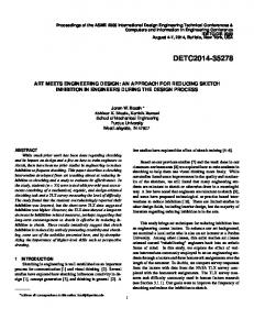
Figure 12. Parallelism profile for Boruvka’s algorithm. Random graph with N = 10,000, node degree uniformly random in [1, 10] and uniformly random edge weights. boruvka-uf-gk shows conflict management with gatekeeping. boruvka-uf-ml shows conflict management with memory-level locking. boruvka-ec shows an alternate implementation of Boruvka’s algorithm that uses edge contraction instead of union-find.

Available Parallelism 1000 2000 3000

7.

boruvka−uf−ml boruvka−uf−gk

kruskal−uf−ml kruskal−uf−gk

239

1148

0

box, we allow the gatekeeper to interact with a data structure’s internal state. In the case of find, for example, the gatekeeper can monitor which nodes are traversed while locating the representative node. If any of these nodes were the “loser” of an active union invocation, a conflict is detected. Hence, the gatekeeper no longer needs to undo unions to check commutativity. This dramatically reduces the amount of time required to verify commutativity conditions, improving performance. The tradeoff to making this optimization is that the gatekeeper is now tightly coupled to the implementation of the data structure, and can only protect this particular implementation. This may be an acceptable tradeoff for performance reasons. Note, however, that this gatekeeper is still compatible with the commutativity specification.

1

5

10 50 100 Computation Step (log−scale)

500

Figure 13. Parallelism profile for Kruskal’s algorithm. Random graph with N = 10,000, node degree uniformly random in [1, 10] and uniformly random edge weights. kruskal-uf-gk shows conflict management with gatekeeping. kruskal-uf-ml shows conflict management with memory-level locking.

Figure 12 shows the available parallelism for Boruvka’s algorithm using two versions of union-find: one protected with memory level locking and one protected with a gatekeeper as described in Section 6. To evaluate the impact of choosing the right data structure, we also implemented a version of Boruvka’s algorithm that does not use a union-find structure at all. This version maintains connected

component information by applying edge contraction directly on the input graph. We union two nodes a and b by removing the edge (a, b), creating a new node c with the same connectivity as a or b and then finally removing a and b from the graph. Commutativity is determined by acquiring abstract locks on nodes of the graph. Boruvka’s with edge contraction has a longer critical path than either union-find variant. With edge contraction, two iterations can process components concurrently only if the components share no outgoing edges. Using a union-find data structure with memorylevel locking to implement Boruvka’s algorithm allows two elements to be processed simultaneously as long as neither accesses data in the union-find data structure that the other modified. The upshot is that many components which share outgoing edges can nevertheless be processed in parallel. In the absence of path compression, memory-level locking and gatekeeping are both compatible with the commutativity conditions in Figure 10. However, under memory-level locking, path compression can conflict with outstanding methods because parent pointers are updated for the entire path from the find argument to its representative node, invalidating other concurrent finds and unions that must traverse the same path. Because each iteration of Boruvka’s algorithm invokes multiple finds, allowing overlapping find invocations to proceed in parallel affords a significant increase in parallelism, as we see in Figure 12. Unsurprisingly, Boruvka’s with gatekeeping has the shortest critical path. We see further evidence of the effect of path compression when we consider Figure 13, which shows the available parallelism in

12

2009/10/5

7.1

Boruvka’s and Kruskal’s Algorithms

Available Parallelism 1000 2000 3000

Figure 15 shows performance results for agglomerative clustering with a kd-tree using gatekeeping. We see reasonable parallel speedup up to 64 threads, which shows the practicality of using gatekeeping to efficiently protect concurrent data structures.

clustering−kd−ml clustering−kd−gk

8.

1040

0

81

1

5

10 50 100 Computation Step (log−scale)

500

Speedup over Sequential 0 5 10 15 20 25

Figure 14. Parallelism profile for agglomerative clustering. Random graph with N = 10,000. clustering-uf-gk shows conflict management using gatekeeping. clustering-uf-ml shows conflict management with memory-level locking.

●

● ● ● ● ●

●

1

2

●

4

8 16 32 Number of Threads

64

128

Figure 15. Performance of agglomerative clustering using gatekeeping conflict management on Sun E25K server running SunOS 5.9. Server consists of 16 CPU boards with four dual-core 1.05 GHz UltraSPARC IV processors. Code compiled with Sun Java compiler version 1.6.0. Each result is the best of 9 runs within the same virtual machine. Speedup relative to sequential implementation. Random graph with N = 500,000. Kruskal’s algorithm, with the two variants of union-find. Kruskal’s is an ordered algorithm, but both Kruskal’s and Boruvka’s algorithm are based around union-find. The difference in computation times is mainly due to the modest bump in available parallelism towards the end of computation. Compared to sequential execution, even a small increase in parallelism can shorten computation time dramatically. Strikingly, while the change in available parallelism between memory-level locking and gatekeeping in Boruvka’s algorithm is large, the change in Kruskal’s algorithm is much smaller. The discrepancy comes from the difference in the mix of methods issued by Boruvka’s and Kruskal’s algorithm. For Boruvka’s, each iteration invokes find for each edge leaving a connected component and then calls union. Kruskal’s, on the other hand, simply invokes find for each endpoint of a single edge and calls union. Boruvka’s algorithm invokes more finds than Kruskal’s, and under memorylevel locking, each find is less likely to commute with other finds or unions.

Related Work

Commutativity conditions can be seen as a highly generalized form of predicate locks as used in databases [6], where locks on arbitrary predicates are used to determine when transactions (in our case, iterations) can successfully execute in parallel. Database research has been the source of a considerable number of techniques to exploit the high level properties of abstract data types, including commutativity, for concurrency control [2, 22, 24]. That work laid the foundation for subsequent work that focused on exploiting data structure semantics in optimistic parallelization and synchronization schemes in shared memory systems [9, 15, 17]. Ni et al attempted to address the shortcomings of memory-level locking as implemented by transactional memory systems by introducing open nesting, which uses abstract locks to synchronize access to data structures by exploiting their semantics [17]. However, the work focuses mainly on the mechanism of integrating abstract locking with a transactional memory, rather than on how to use abstract locks in data structures in a disciplined manner. In fact, the authors note that improper use of open nesting could lead to deadlock situations. Herlihy and Koskinen proved that commutativity information informs a disciplined, safe approach for implementing open nesting [9]. They boost data structures, by adding abstract locks to implement a restricted form of commutativity, providing structures with the benefits of open nesting but no possibility of deadlock. There are two significant differences between [9] and our work. First, while Herlihy and Koskinen describe boosting as a general scheme which allows arbitrary code to be executed to detect semantic conflicts, they provide little intuition as to how this conflict detection should occur; in many of their examples, they use abstract locks to implement boosting even though they do not take full advantage of commutativity. In contrast, our work provides two systematic approaches for constructing commutativity checkers (via abstract locking or gatekeeping), each with well-defined expressive power. Second, Boosting is validated by evaluating particular locking implementations. In contrast, our results quantify, in an implementation-independent manner, the parallelism exposed by higher-level conflict detection. This paper builds most directly on the work of Kulkarni et al. who showed that considering commutativity is important to building an efficient system for optimistically parallelizing amorphous data-parallel applications [15]. Our implementation of gatekeepers is inspired by the scheme sketched out in their work. However, the authors do not quantify the benefits of using commutativity conditions as opposed to more straightforward approaches such as memory-level locking.

9.

Future work and Conclusions

Figure 14 shows the available parallelism of agglomerative clustering using a kd-tree. Under memory-level locking, add, remove, and nearest invocations conflict with each other whenever the metadata of the kd-tree is modified. Under gatekeeping, these methods commute as long as they do not invalidate any outstanding nearest invocations. Because agglomerative clustering performs numerous nearest invocations, we see that gatekeeping provides a substantial boost in parallelism compared to memory-level locking.

There are a number of promising directions for future research. First, in this paper we make no attempt to prove the correctness of commutativity conditions. It would be interesting to determine what information about the abstract state of a data structure is required to verify that commutativity conditions correctly obey Definition 9. Second, for data structures such as union-find, determining appropriate commutativity conditions is difficult; is there a way to generate commutativity conditions given a data structure specification? Finally, there are also interesting avenues of implementation research: although gatekeepers are expressive, they are often quite inefficient. Are there more efficient conflict detection schemes that

13

2009/10/5

7.2

Agglomerative Clustering

do not overly sacrifice expressibility? Can efficient gatekeepers be synthesized from commutativity conditions, similar to how we synthesize abstract locking schemes? This work formalized the concept of commutativity conditions and showed how the commutativity of methods on data structures can be used to guarantee the correct parallel execution of programs exhibiting amorphous data-parallelism. We discussed two prior approaches to achieving parallel execution, memory-level locking and abstract locking, and provided sufficient conditions on commutativity conditions which explain when these approaches can capture all the parallelism that is available in a program. We also presented a new conflict detection approach, called gatekeeping, which can completely capture a commutativity specification and thus find the maximum amount of parallelism the specification allows. We observed that fully exploiting commutativity by using gatekeeping can lead to a significant increase in the amount of parallelism found in amorphous data-parallel programs, and demonstrated that, for one application, gatekeepers could be used to efficiently exploit commutativity to obtain significant parallel speedup.

[14]

[15]

[16]

[17]

[18] [19]

References [1] Philip A. Bernstein, Vassoso Hadzilacos, and Nathan Goodman. Concurrency control and recovery in database systems. AddisonWesley Longman Publishing Co., Inc., Boston, MA, USA, 1987. [2] A. Bondavalli, N. De Francesco, D. Latella, and G. Vaglini. Shared abstract data type: an algebraic methodology for their specification. In MFDBS 89: Proceedings of the second symposium on Mathematical fundamentals of database systems, pages 53–67, New York, NY, USA, 1989. Springer-Verlag New York, Inc. [3] Brian D. Carlstrom, Austen McDonald, Hassan Chafi, JaeWoong Chung, Chi Cao Minh, Christos Kozyrakis, and Kunle Olukotun. The atomos transactional programming language. SIGPLAN Not., 41(6):1–13, 2006. [4] Brian D. Carlstrom, Austen McDonald, Christos Kozyrakis, and Kunle Olukotun. Transactional collection classes. In Principles and Practices of Parallel Programming (PPoPP), 2007. [5] Thomas Cormen, Charles Leiserson, Ronald Rivest, and Clifford Stein, editors. Introduction to Algorithms. MIT Press, 2001. [6] K. P. Eswaran, J. N. Gray, R. A. Lorie, and I. L. Traiger. The notions of consistency and predicate locks in a database system. Commun. ACM, 19(11):624–633, 1976. [7] Jim Gray and Andreas Reuter. Transaction Processing: Concepts and Techniques. Morgan Kaufmann Publishers Inc., San Francisco, CA, USA, 1992. [8] Lance Hammond, Vicky Wong, Mike Chen, Brian D. Carlstrom, John D. Davis, Ben Hertzberg, Manohar K. Prabhu, Honggo Wijaya, Christos Kozyrakis, and Kunle Olukotun. Transactional memory coherence and consistency. ISCA, 00:102, 2004. [9] Maurice Herlihy and Eric Koskinen. Transactional boosting: a methodology for highly-concurrent transactional objects. In PPoPP ’08: Proceedings of the 13th ACM SIGPLAN Symposium on Principles and practice of parallel programming, 2008. [10] Maurice Herlihy, Victor Luchangco, Mark Moir, and William N. Scherer, III. Software transactional memory for dynamic-sized data structures. In PODC ’03: Proceedings of the twenty-second annual symposium on Principles of distributed computing, 2003. [11] Maurice P. Herlihy and Jeannette M. Wing. Linearizability: a correctness condition for concurrent objects. ACM Transactions on Programming Languages and Systems (TOPLAS), 12(3):463–492, 1990. [12] Venkata Krishnan and Josep Torrellas. A chip-multiprocessor architecture with speculative multithreading. IEEE Trans. Comput., 48(9):866–880, 1999. [13] Milind Kulkarni, Martin Burtscher, Rajeshkar Inkulu, Keshav Pingali, and Calin Casc¸aval. How much parallelism is there in irregular applications? In PPoPP ’09: Proceedings of the 14th ACM SIGPLAN

14

[20]

[21]

[22] [23]

[24]

symposium on Principles and practice of parallel programming, 2009. Milind Kulkarni, Keshav Pingali, Ganesh Ramanarayanan, Bruce Walter, Kavita Bala, and L. Paul Chew. Optimistic parallelism benefits from data partitioning. SIGARCH Comput. Archit. News (Proceedings of ASPLOS 2008), 36(1):233–243, 2008. Milind Kulkarni, Keshav Pingali, Bruce Walter, Ganesh Ramanarayanan, Kavita Bala, and L. Paul Chew. Optimistic parallelism requires abstractions. SIGPLAN Not. (Proceedings of PLDI 2007), 42(6):211–222, 2007. Kevin E. Moore, Jayaram Bobba, Michelle J. Moravan, Mark D. Hill, and David A. Wood. Logtm: Log-based transactional memory. In HPCA ’06: Proceedings of the 12th International Symposium on High Performance Computer Architecture, 2006. Yang Ni, Vijay Menon, Ali-Reza Adl-Tabatabai, Antony L. Hosking, Rick Hudson, J. Eliot B. Moss, Bratin Saha, and Tatiana Shpeisman. Open nesting in software transactional memory. In Principles and Practices of Parallel Programming (PPoPP), 2007. Christos H. Papadimitriou. The serializability of concurrent database updates. J. ACM, 26(4):631–653, 1979. Lawrence Rauchwerger and David A. Padua. The LRPD test: Speculative run-time parallelization of loops with privatization and reduction parallelization. IEEE Trans. Parallel Distrib. Syst., 10(2):160–180, 1999. Bratin Saha, Ali-Reza Adl-Tabatabai, Richard L. Hudson, Chi Cao Minh, and Benjamin Hertzberg. McRT-STM: a high performance software transactional memory system for a multi-core runtime. In PPoPP ’06: Proceedings of the eleventh ACM SIGPLAN symposium on Principles and practice of parallel programming, pages 187–197, New York, NY, USA, 2006. ACM Press. Hanan Samet. Foundations of Multidimensional and Metric Data Structures (The Morgan Kaufmann Series in Computer Graphics and Geometric Modeling). Morgan Kaufmann Publishers Inc., San Francisco, CA, USA, 2005. Peter M. Schwarz and Alfred Z. Spector. Synchronizing shared abstract types. ACM Trans. Comput. Syst., 2(3):223–250, 1984. Bruce Walter, Kavita Bala, Milind Kulkarni, and Keshav Pingali. Fast agglomerative clustering for rendering. In Interactive Ray Tracing, 2008. RT 2008. IEEE Symposium on, pages 81–86, Aug. 2008. W.E. Weihl. Commutativity-based concurrency control for abstract data types. IEEE Transactions on Computers, 37(12), 1988.

2009/10/5