An Effective Fixpoint Semantics for Linear Logic Programs

arXiv:cs/0102025v2 [cs.PL] 23 Mar 2001

Under consideration for publication in Theory and Practice of Logic Programming

1

An Effective Fixpoint Semantics for Linear Logic Programs MARCO BOZZANO, GIORGIO DELZANNO and MAURIZIO MARTELLI Dipartimento di Informatica e Scienze dell’Informazione Universit` a di Genova Via Dodecaneso 35, 16146 Genova - Italy (e-mail: {bozzano,giorgio,martelli}@disi.unige.it)

Abstract In this paper we investigate the theoretical foundation of a new bottom-up semantics for linear logic programs, and more precisely for the fragment of LinLog (Andreoli, 1992) that consists of the language LO (Andreoli & Pareschi, 1991) enriched with the constant 1. We use constraints to symbolically and finitely represent possibly infinite collections of provable goals. We define a fixpoint semantics based on a new operator in the style of TP working over constraints. An application of the fixpoint operator can be computed algorithmically. As sufficient conditions for termination, we show that the fixpoint computation is guaranteed to converge for propositional LO. To our knowledge, this is the first attempt to define an effective fixpoint semantics for linear logic programs. As an application of our framework, we also present a formal investigation of the relations between LO and Disjunctive Logic Programming (Minker et al., 1991). Using an approach based on abstract interpretation, we show that DLP fixpoint semantics can be viewed as an abstraction of our semantics for LO. We prove that the resulting abstraction is correct and complete (Cousot & Cousot, 1977; Giacobazzi & Ranzato, 1997) for an interesting class of LO programs encoding Petri Nets.

1 Introduction In recent years a number of fragments of linear logic (Girard, 1987) have been proposed as a logical foundation for extensions of logic programming(Miller, 1995). Several new programming languages like LO (Andreoli & Pareschi, 1991), LinLog (Andreoli, 1992), ACL (Kobayashi & Yonezawa, 1995), Lolli (Hodas & Miller, 1994), and Lygon (Harland & Pym, 1994) have been proposed with the aim of enriching traditional logic programming languages like Prolog with a well-founded notion of state and with aspects of concurrency. The operational semantics of this class of languages is given via a sequent-calculi presentation of the corresponding fragment of linear logic. Special classes of proofs like the focusing proofs of (Andreoli, 1992) and the uniform proofs of (Miller, 1996) allow us to restrict our attention to cutfree, goal-driven proof systems that are complete with respect to provability in linear logic. These presentations of linear logic are the natural counterpart of the traditional top-down operational semantics of logic programs. In this paper we investigate an alternative operational semantics for the fragment

2

M. Bozzano, G. Delzanno and M. Martelli

of linear logic underlying the language LO (Andreoli & Pareschi, 1991), and its proper extension with the constant 1. Both languages can be seen as fragments of LinLog (Andreoli, 1992), which is a presentation of full linear logic. Throughout the paper, we will simply refer to these two fragments as LO and LO1 . The reason we selected these fragments is that we were looking for a relatively simple linear logic language with a uniform-proof presentation, state-based computations and aspects of concurrency. Considering both LO and its extension with the constant 1 will help us to formally classify the different expressive power of linear logic connectives like ................. ........ ..., & , ⊤, and 1 when incorporated into a logic programming setting. In practice, LO has been successfully applied to model concurrent object-oriented languages (Andreoli & Pareschi, 1991), and multi-agent coordination languages based on the Linda model (Andreoli, 1996). The operational semantics we propose consists of a goal-independent bottom-up evaluation of programs. Specifically, given an LO program P our aim is to compute a finite representation of the set of goals that are provable from P . There are several reasons to look at this problem. First of all, as discussed in (Harland & Winikoff, 1998), the bottom-up evaluation of programs is the key ingredient for all applications where it is difficult or impossible to specify a given goal in advance. Examples are active (constraint) databases, agent-based systems and genetic algorithms. Recent results connecting verification techniques and semantics of logic programs (Delzanno & Podelski, 1999) show that bottom-up evaluation can be used to automatically check properties (specified in temporal logic like CTL) of the original program. In this paper will go further showing that the provability relation in logic programming languages like LO can be used to naturally express verification problems for Petri Nets-like models of concurrent systems. Finally, a formal definition of the bottom-up semantics can be useful for studying equivalence, compositionality and abstract interpretation, as for traditional logic programs (Bossi et al., 1994; Gabbrielli et al., 1995). Technically, our contributions are as follows. We first consider a formulation of ........... LO with ................., −◦, & and ⊤. Following the semantic framework of (constraint) logic programming (Gabbrielli et al., 1995; Jaffar & Maher, 1994), we formulate the bottom-up evaluation procedure in two steps. We first define what one could call a ground semantics via a fixpoint operator TP defined over an extended notion of Herbrand interpretation consisting of multisets of atomic formulas. This way, we capture the uniformity of LO-provability, according to which compound goals must be completely decomposed into atomic goals before program clauses can be applied. Due to the structure of the LO proof system, already in the propositional case there are infinitely many provable multisets of atomic formulas. In fact, LOprovability enjoys the following property. If a multiset of goals ∆ is provable in P , then any ∆′ such that ∆ is a sub-multiset of ∆′ is provable in P . To circumvent this problem, we order the interpretations according to the multiset inclusion relation of their elements and we define a new operator SP that computes only the minimal (w.r.t. multiset inclusion) provable multisets. Dickson’s Lemma (Dickson, 1913) ensures the termination of the fixpoint computation based on SP for propositional LO programs. Interestingly, this result is an instance of the general decidability

Fixpoint Semantics for Linear Logic Programs

3

results for model checking of infinite-state systems given in (Abdulla et al., 1996; Finkel & Schnoebelen, 2001). The decidability of propositional provability shows that LO is not as interesting as one could expect from a state-oriented extension of the logic programming paradigm. Specifically, LO does not provide a natural way to count resources. This feature can be introduced by a slight extension of LO in which we add unit clauses defined via the constant 1. The resulting language, namely LO1 , can be viewed as a first step towards more complex languages based on linear logic like LinLog (Andreoli, 1992). As we show in this paper, LO1 allows to model more sophisticated models of concurrent systems than LO, e.g., in LO1 it is possible to model Petri Nets with transfer arcs. Adding the constant 1 breaks down the decidability of provability in propositional LO. Despite this negative result, it is still possible to define an effective SP1 operator for LO1 . For this purpose, as symbolic representation of potentially infinite sets of contexts, we choose a special class of linear constraints defined over variables that count resources. This abstract domain generalizes the domain used for LO: the latter can be represented as the subclass of constraints with no equalities. Though for the new operator we cannot guarantee that the fixpoint can be reached after finitely many steps, this connection allows us to apply techniques developed in model checking for infinite-state systems (see e.g. (Bultan et al., 1997; Delzanno & Podelski, 1999; Henzinger et al., 1997)) and abstract interpretation (Cousot & Halbwachs, 1978) to compute approximations of the fixpoint of SP1 . In this paper we limit ourselves to the study of the propositional case that, as shown in (Andreoli et al., 1997), can be viewed as the target of a possible abstract interpretation of a first-order program. To our knowledge, this is the first attempt of defining an effective fixpoint semantics for linear logic programs. Our semantic framework can also be used as a tool to compare the relative strength of different logic programming extensions. As an application, we shall present a detailed comparison between LO and Disjunctive Logic Programming (DLP). Though DLP has been introduced in order to represent ‘uncertain’ beliefs, a closer look at its formal definition reveals very interesting connections with the paradigm of linear logic programming: both DLP and LO programs extend Horn programs allowing clauses with multiple heads. In fact, in DLP we find clauses of the form p(X ) ∨ q(X ) ← r (X ) ∧ t (X ), whereas in LO we find clauses of the form p(X )

............... .......... ...

q(X ) ◦− r (X ) & t (X )·

To understand the differences, we must look at the operational semantics of DLP programs. In DLP, a resolution step is extended so as to work over positive clauses (sets/disjunctions of facts). Implicit contraction steps are applied over the selected clause. On the contrary, being in a sub-structural logic in which contraction is forbidden, we know that LO resolution behaves as multiset rewriting. Following the bottom-up approach that we pursue in this paper, we will exploit the classical frame-

4


work of abstract interpretation to formally compare the two languages. Technically, we first specialize our fixpoint semantics to a flat fragment of propositional LO (i.e., arbitrary nesting of connectives in goals is forbidden) which directly corresponds to DLP as defined in (Minker et al., 1991). Then, by using an abstract-interpretationbased approach, we exhibit a Galois connection between the semantic domains of DLP and LO, and we show that the semantics of DLP programs can be described as an abstraction of the semantics of LO programs. Using the theory of abstract interpretation and the concept of complete abstraction (Cousot & Cousot, 1977; Giacobazzi & Ranzato, 1997) we discuss the quality of the resulting abstraction. This view of DLP as an abstraction of LO is appealing for several reasons. First of all, it opens the possibility of using techniques developed for DLP for the analysis of LO programs. Furthermore, it shows that the paradigm of DLP could have unexpected applications as a framework to reason about properties of Petri Nets, a well-know formalism for concurrent computations (Karp & Miller, 1969). In fact, as we will prove formally in the paper, DLP represents a complete abstract domain for LO programs that encode Petri Nets. Plan of the paper. After introducing some notations in Section 2, in Section 3 we recall the main features of LO (Andreoli & Pareschi, 1991). In Section 4 we introduce the so-called ground semantics, via the TP operator, and prove that the least fixpoint of TP characterizes the operational semantics of an LO program. In Section 5 we reformulate LO semantics by means of the symbolic SP operator, and we relate it to TP . In Section 6 we consider an extended fragment of LO with the constant 1, extending the notion of satisfiability given in Section 4 and introducing an operator TP1 . In Section 7 we introduce a symbolic operator SP1 for the extended fragment, and we discuss its algorithmic implementation in Section 8. As an application of our framework, in Section 9 and Section 10 we investigate the relations between LO and DLP, and in Section 11 we investigate the relations with Petri Nets. Finally, in Section 12 and Section 13 we discuss related works and conclusions. This paper is an extended version of the papers (Bozzano et al., 2000a; Bozzano et al., 2000b). 2 Preliminaries In this paper we will extensively use operations on multisets. We will consider a fixed signature, i.e a finite set of propositional symbols, Σ = {a1 , . . . , an }. Multisets over Σ will be hereafter called facts, and symbolically noted as A, B, C, . . .. A multiset with (possibly duplicated) elements b1 , . . . , bm ∈ Σ will be simply indicated as {b1 , . . . , bm }, overloading the usual notation for sets. A fact A is uniquely determined by a finite map Occ : Σ → N such that OccA (ai ) is the number of occurrences of ai in A. Facts are ordered according to the multiset inclusion relation 4 defined as follows: A 4 B if and only if OccA (ai ) ≤ OccB (ai ) for i : 1, . . . , n. The empty multiset is denoted ǫ and is such that Occǫ (ai ) = 0 for i : 1, . . . , n, and ǫ 4 A for any A. The multiset union A, B (alternatively


5

A + B when ‘,’ is ambiguous) of two facts A and B is such that OccA,B (ai ) = OccA (ai ) + OccB (ai ) for i : 1, . . . , n. The multiset difference A \ B is such that OccA\B (ai ) = max (0, OccA (ai ) − OccB (ai )) for i : 1, . . . , n. We define a special operation • to compute the least upper bound of two facts with respect to 4. Namely, A • B is such that OccA•B (ai ) = max (OccA (ai ), OccB (ai )) for i : 1, . . . , n. Finally, we will use the notation An , where n is a natural number, to indicate A + . . . + A (n times). In the rest of the paper we will use ∆, Θ, . . . to denote multisets of possibly compound formulas. Given two multisets ∆ and Θ, ∆ 4 Θ indicates multiset inclusion and ∆, Θ multiset union, as before, and ∆, {G} is written simply ∆, G. In the following, a context will denote a multiset of goal-formulas (a fact is a context in which every formula is atomic). Given a linear disjunction of atomic formulas ........... ........... b to denote the multiset a1 , . . . , an . H = a1 ................. . . . ................ an , we introduce the notation H Finally, let T : I → I be an operator defined over a complete lattice hI, ⊑i. We define T↑0 = ∅, where ∅ is the bottom element, T↑k +1 = T (T↑k ) for all k ≥ 0, and F∞ F T↑ω = k =0 T↑k , where is the least upper bound w.r.t. ⊑. Furthermore, we use lf p(T ) to denote the least fixpoint of T . 3 The Programming Language LO LO (Andreoli & Pareschi, 1991) is a logic programming language based on linear logic. Its mathematical foundations lie on a proof-theoretical presentation of a fragment of linear logic defined over the linear connectives ◦− (linear implication), & ........... (additive conjunction), ............... (multiplicative disjunction), and the constant ⊤ (additive identity). In the propositional case LO consists of the following class of formulas: D ::= A1

................ ........ ....

...

............... .......... ...

An ◦− G | D & D

............

G ::= G ................. G | G & G | A | ⊤ Here A1 , . . . , An and A range over propositional symbols from a fixed signature Σ. G-formulas correspond to goals to be evaluated in a given program. D-formulas correspond to multiple-headed program clauses. An LO program is a D-formula. Let P be the program C1 & . . . & Cn . The execution of a multiset of G-formulas G1 , . . . , Gk in P corresponds to a goal-driven proof for the two-sided LO-sequent P ⇒ G1 , . . . , Gk · The LO-sequent P ⇒ G1 , . . . , Gk is an abbreviation for the following two-sided linear logic sequent: !C1 , . . . , !Cn → G1 , . . . , Gk · The formula !F on the left-hand side of a sequent indicates that F can be used in a proof an arbitrary number of times. This implies that an LO-Program can be viewed also as a set of reusable clauses. According to this view, the operational semantics of LO is given via the uniform (goal-driven) proof system defined in Figure 1. In Figure 1, P is a set of implicational clauses, A denotes a multiset of atomic formulas, whereas ∆ denotes a multiset of G-formulas. A sequent is provable if all branches

6

M. Bozzano, G. Delzanno and M. Martelli P ⇒ G1 , G2 , ∆ P ⇒ ⊤, ∆

⊤r

................. ...... 1 .....

P ⇒G

.............. .......... ...r

P ⇒ G1 , ∆

P ⇒ G2 , ∆

P ⇒ G1 & G2 , ∆

G2 , ∆

&r

P ⇒ G, A bc (H ◦− G ∈ P ) b +A P ⇒H

Fig. 1. A proof system for LO

of its proof tree terminate with instances of the ⊤r axiom. The proof system of Figure 1 is a specialization of more general uniform proof systems for linear logic like Andreoli’s focusing proofs (Andreoli, 1992), and Forum (Miller, 1996). The b is the multiset consisting of the rule bc denotes a backchaining (resolution) step (H literals in the disjunction H , see Section 2). Note that bc can be executed only if the right-hand side of the current LO sequent consists of atomic formulas. Thus, LO clauses behave like multiset rewriting rules. LO clauses having the following form a1

................. ........ ...

...

................. ........ ...

an ◦− ⊤

play the same role as the unit clauses of Horn programs. In fact, a backchaining step over such a clause leads to success independently of the current context A, as shown in the following scheme: P ⇒ ⊤, A

⊤r

P ⇒ a1 , . . . , an , A provided

a1

.............. .......... ...

...

.............. .......... ...

bc

an ◦− ⊤ ∈ P

This observation leads us to the following property (we recall that 4 is the submultiset relation). Proposition 1 Given an LO program P and two contexts ∆, ∆′ such that ∆ 4 ∆′ , if P ⇒ ∆ then P ⇒ ∆′ . Proof By simple induction on the structure of LO proofs. This property is the key point in our analysis of the operational behavior of LO. It states that the weakening rule is admissible in LO. Thus, LO can be viewed as an affine fragment of linear logic. Note that weakening and contraction are both admissible on the left hand side (i.e. on the program part) of LO sequents. Example 1

Fixpoint Semantics for Linear Logic Programs ⊤r

P ⇒ e, ⊤

bc (3)

P ⇒ d , e, c P ⇒d

............... ......... ....

7

P ⇒⊤

............... ......... ...r

P ⇒ f,c

e, c

P ⇒ (d

............... ........ ..

bc (5) &r

e) & f , c bc (2)

P ⇒ b, c P ⇒b

⊤r

............. .......... ...

............... .......... ...r

c

P ⇒ e, e

bc (4)

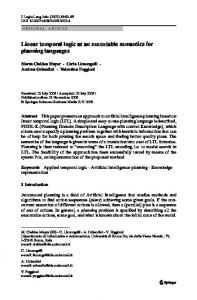
Fig. 2. An LO proof for the goal e, e in the program of Example 1 Let P be the LO program consisting of the clauses 1· 2· 3· 4· 5·

...........

a ◦− b ................ c ............ b ◦− (d ................ e) & f ................ c ........... d ◦− ⊤ .......... ........... e ................. e ◦− b ................. c . . . . . . . .. .. c ................ f ◦− ⊤

and consider an initial goal e, e. A proof for this goal is shown in Figure 2, where we have denoted by bc (i) the application of the backchaining rule over clause number i of P . The proof proceeds as follows. Using clause 4., to prove e, e we have to prove ............ ........... b ................ c, which, by LO ................r rule, reduces to prove b, c. At this point we can backchain ........... over clause 2., and we get the new goal (d ................. e) & f , c. By applying & r rule, we ............ ............... get two separate goals d ............ e, c and f , c. The first, after a reduction via ................r rule, is provable by means of clause (axiom) 3., while the latter is provable directly by clause (axiom) 5. Note that ⊤ succeeds in a non-empty context (i.e. containing e) in the left branch. A similar proof shows that the goal a is also provable from P . By Proposition 1, provability of e, e and a implies provability of any multiset of goals e, e, ∆ and a, ∆, for every context ∆. 2 We conclude this Section with the definition of the following induction measure on LO goals, which we will later need in proofs. Definition 3.1 Given a goal G, the induction measure m(G) is defined according to the following ........... rules: m(A) = 0 for every atomic formula A; m(⊤) = 0; m(G1 & G2 ) = m(G1 ................ G2 ) = m(G1 ) + m(G2 ) + 1. The induction measure extends to contexts by defining m(G1 , . . . , Gn ) = m(G1 ) + . . . + m(Gn ). 4 A Bottom-up Semantics for LO The proof-theoretical semantics of LO corresponds to the top-down operational semantics based on resolution for traditional logic programming languages like Prolog. Formally, we define the operational top-down semantics of an LO program P

8


as follows: O (P ) = {A | A is a fact and P ⇒ A is provable} Note that the information on provable facts from a given program P is all we need to decide whether a general goal (with possible nesting of connectives) is provable from P or not. This is a consequence of the focusing property (Andreoli, 1992) of LO provability, which ensures that provability of a compound goal can always be reduced to provability of a finite set of atomic multisets. In a similar way, in Prolog the standard bottom-up semantics is defined as a set of atoms, while in general conjunctions of atoms are allowed in clause bodies. In this paper we are interested in finding a suitable definition of bottom-up semantics that can be used as an alternative operational semantics for LO. More precisely, given an LO program P we would like to define a procedure to compute all goal formulas G such that G is provable from P . This procedure should enjoy the usual properties of classical bottom-up semantics, in particular its definition should be based on an effective fixpoint operator (i.e. at least every single step must be finitely computable), and it should be goal-independent. As usual, goal independence is achieved by searching for proofs starting from the axioms (the unit clauses of Section 3) and accumulating goals which can be proved by applying program clauses to the current interpretation. As for the operational semantics, we can limit ourselves to goal formulas consisting of multisets of atomic formulas, without any loss of generality. In the rest of the paper we will always consider propositional LO programs defined over a finite set of propositional symbols Σ. We give the following definitions. Definition 4.1 (Herbrand base BP ) Given a propositional LO program P defined over Σ, the Herbrand base of P , denoted BP , is given by BP = {A | A is a multiset (fact) over Σ}· Definition 4.2 (Herbrand interpretation) We say that I ⊆ BP is a Herbrand interpretation. Herbrand interpretations form a complete lattice hD, ⊆i with respect to set inclusion, where D = P(BP ). Before introducing the formal definition of the ground bottom-up semantics, we need to define a notion of satisfiability of a context ∆ in a given interpretation I . For this purpose, we introduce the judgment I |= ∆[A]. The need for this judgment, with respect to the familiar logic programming setting (Gabbrielli et al., 1995), is motivated by the arbitrary nesting of connectives in LO clause bodies, which is not allowed in traditional presentations of (constraint) logic programs. In I |= ∆[A], A should be read as an output fact such that A + ∆ is valid in I . This notion of satisfiability is modeled according to the right-introduction rules of the connectives. The notion of output fact A will simplify the presentation of the algorithmic version of the judgment which we will present in Section 5. Definition 4.3 (Satisfiability)


9

Let I be a Herbrand interpretation, then |= is defined as follows: I |= ⊤, ∆[A′ ] for any fact A′ ; I |= A[A′ ] if A + A′ ∈ I ; I |= G1

............... .......... ...

G2 , ∆[A] if I |= G1 , G2 , ∆[A];

I |= G1 & G2 , ∆[A] if I |= G1 , ∆[A] and I |= G2 , ∆[A]· The relation |= satisfies the following properties. Lemma 1 For any interpretations I , J , context ∆, and fact A, i) I |= ∆[A] if and only if I |= ∆, A[ǫ]; ii) if I ⊆ J and I |= ∆[A] then J |= ∆[A]; S∞ iii) given a chain of interpretations I1 ⊆ I2 ⊆ . . ., if i=1 Ii |= ∆[A] then there exists k s.t. Ik |= ∆[A]. Proof The proof of i) and ii) is by simple induction. The proof of iii) is by (complete) induction on m(∆) (see Definition 3.1). - If ∆ = ⊤, ∆′ , then, no matter which k you choose, Ik |= ⊤, ∆′ [A]; S S∞ - if ∆ is a fact, then ∞ i=1 Ii |= ∆[A] means ∆, A ∈ i=1 Ii , which in turn implies that there exists k such that ∆, A ∈ Ik , therefore Ik |= ∆[A]; - if ∆ = G1 & G2 , ∆′ , then by inductive hypothesis there exist k1 and k2 s.t. Ik1 |= G1 , ∆′ [A] and Ik2 |= G2 , ∆′ [A]. Therefore, if k = max {k1 , k2 }, by ii) we have that Ik |= G1 , ∆′ [A] and Ik |= G2 , ∆′ [A], therefore Ik |= G1 & G2 , ∆′ [A], i.e. Ik |= ∆[A] as required; ........... - the ...............-case follows by a straightforward application of the inductive hypothesis.

We now come to the definition of the fixpoint operator TP . Definition 4.4 (Fixpoint operator TP ) Given a program P and an interpretation I , the operator TP is defined as follows: b + A | H ◦− G ∈ P , I |= G[A]}· TP (I ) = {H The following property holds. Proposition 2 For every program P , Tp is monotonic and continuous over the lattice hD, ⊆i. Proof Monotonicity. Immediate from TP definition and Lemma 1 ii). Continuity. We prove that TP is finitary. Namely, given an increasing chain of S∞ S∞ interpretations I1 ⊆ I2 ⊆ . . ., TP is finitary if TP ( i=1 Ii ) ⊆ i=1 TP (Ii ). We S∞ simply need to show that if TP ( i=1 Ii ) |= ∆[ǫ] then there exists k such that TP (Ik ) |= ∆[ǫ]). The proof is by induction on m(∆).

10

M. Bozzano, G. Delzanno and M. Martelli - If ∆ = ⊤, ∆′ , then, no matter which k you choose, TP (Ik ) |= ⊤, ∆′ [ǫ]; S∞ - if ∆ is a fact and ∆ ∈ TP ( i=1 Ii ), then, by definition of TP , there exist S∞ .......... .............. a fact A and a clause A1 ............. . . . ................. An ◦− G ∈ P , such that i=1 Ii |= G[A] and ∆ = A1 , . . . , An , A. Lemma 1 iii) implies that ∃k · Ik |= G[A], therefore, again by definition of TP , TP (Ik ) |= A1 , . . . , An , A[ǫ], i.e. TP (Ik ) |= ∆[ǫ] as required; - if ∆ = G1 & G2 , ∆′ , then by inductive hypothesis, there exist k1 and k2 s.t. TP (Ik1 ) |= G1 , ∆′ [ǫ] and TP (Ik2 ) |= G2 , ∆′ [ǫ]. Then, if k = max {k1 , k2 }, by Lemma 1 ii) we have that TP (Ik ) |= G1 , ∆′ [ǫ] and TP (Ik ) |= G2 , ∆′ [ǫ]. This implies TP (Ik ) |= G1 & G2 , ∆′ [ǫ], i.e. TP (Ik ) |= ∆[ǫ] as required; .......... - the .................-case follows by a straightforward application of the inductive hypothesis.

Monotonicity and continuity of the TP operator imply, by Tarski’s Theorem, that lf p(TP ) = TP ↑ω . Following (Lloyd, 1987), we define the fixpoint semantics F (P ) of an LO program P as the least fixpoint of TP , namely F (P ) = lf p(TP ). Intuitively, TP (I ) is the set of immediate logical consequences of the program P and of the facts in I . In b ∈ I }, the definition of TP can be fact, if we define PI as the program {A ◦− ⊤ | A viewed as the following instance of the cut rule of linear logic: !P , G → H

!PI → G, A

!P , !PI → H , A

cut

Using the notation used for LO-sequents we obtain the following rule: P ⇒ H ◦− G

PI ⇒ G, A

P ∪ PI ⇒ H , A

cut

Note that, since H ◦− G ∈ P , the sequent P ⇒ H ◦− G is always provable in linear logic. According to this view, F (P ) characterizes the set of logical consequences of a program P . The fixpoint semantics is sound and complete with respect to the operational semantics as stated in the following theorem. Theorem 1 (Soundness and Completeness) For every LO program P , F (P ) = O (P ). Proof i) F (P ) ⊆ O (P ). We prove that for every k and context ∆, if TP ↑k |= ∆[ǫ] then P ⇒ ∆. The proof is by (complete) induction on m(T ¯ P ↑k , ∆), where m ¯ is an induction measure defined by m(T ¯ P ↑k , ∆) = hk , m(∆)i, and hk , mi < hk ′ , m ′ i if and only if (k < k ′ ) or (k = k ′ and m < m ′ ) (lexicographic ordering). - If ∆ = ⊤, ∆′ , the conclusion is immediate; - if ∆ is a fact, then ∆ ∈ TP ↑k , so that TP ↑k 6= ∅ and k > 0. By definition of TP ........... ........... we have that there exist a fact A and a clause A1 ................. . . . ................. An ◦− G ∈ P , such


11

that TP ↑k −1 |= G[A] and ∆ = A1 , . . . , An , A. By Lemma 1 i) we have that TP ↑k −1 |= G, A[ǫ], and then, by inductive hypothesis, P ⇒ G, A, therefore by LO bc rule, P ⇒ A1 , . . . , An , A, i.e., P ⇒ ∆; - if ∆ = G1 & G2 , ∆′ then by inductive hypothesis P ⇒ G1 , ∆′ and P ⇒ G2 , ∆′ , therefore P ⇒ G1 & G2 , ∆′ by LO & r rule; ........... - the ................-case follows by a straightforward application of the inductive hypothesis. ii) O (P ) ⊆ F (P ). We prove that for every context ∆ if P ⇒ ∆ then there exists k such that TP ↑k |= ∆[ǫ] by induction on the structure of the LO proof. - If the proof ends with an application of ⊤r , then the conclusion is immediate; - if the proof ends with an application of the bc rule, then ∆ = A1 , . . . , An , A, ............ ............ where A1 , . . . , An are atomic formulas, and there exists a clause A1 .............. . . . ............. An ◦− G ∈ P . For the uniformity of LO proofs, we can suppose A to be a fact. By inductive hypothesis, we have that there exists k such that TP ↑k |= G, A[ǫ], then, by Lemma 1 i), TP ↑k |= G[A], which, by definition of TP , in turn implies that A1 , . . . , An , A ∈ TP (TP ↑k ) = TP ↑k +1 , therefore TP ↑k +1 |= A1 , . . . , An , A[ǫ], i.e., TP ↑k +1 |= ∆[ǫ]; - if the proof ends with an application of the & r rule, then ∆ = G1 & G2 , ∆′ and, by inductive hypothesis, there exist k1 and k2 such that TP ↑k1 |= G1 , ∆′ [ǫ] and TP ↑k2 |= G2 , ∆′ [ǫ]. Then, if k = max {k1 , k2 } we have, by Lemma 1 ii), that TP ↑k |= G1 , ∆′ [ǫ] and TP ↑k |= G2 , ∆′ [ǫ], therefore TP ↑k |= G1 & G2 , ∆′ [ǫ], i.e. TP ↑k |= ∆[ǫ]; ........... - the ...............-case follows by a straightforward application of the inductive hypothesis. We note that it is also possible to define a model-theoretic semantics (as for classical logic programming (Gabbrielli et al., 1995)) based on the notion of least model with respect to a given class of models and partial order relation. In our setting, the partial order relation is simply set inclusion, while models are exactly Herbrand interpretations which satisfy program clauses, i.e., I is a model of P if and only if for every clause H ◦− G ∈ P and for every fact A, I |= G[A] implies I |= H [A]· It turns out that the operational, fixpoint and model-theoretic semantics are all equivalent. We omit details. Finally, we also note that these semantics can be proved equivalent to the phase semantics for LO given in (Andreoli & Pareschi, 1991). 5 An Effective Semantics for LO The operator TP defined in the previous section does not enjoy one of the crucial properties we required for our bottom-up semantics, namely its definition is not effective. As an example, take the program P consisting of the clause a ◦− ⊤. Then, TP (∅) is the set of all multisets with at least one occurrence of a, which is an infinite set. In other words, TP (∅) = {B | a 4 B }, where 4 is the multiset inclusion relation

12


of Section 2. In order to compute effectively one step of TP , we have to find a finite representation of potentially infinite sets of facts (in the terminology of (Abdulla et al., 1996), a constraint system). The previous example suggests us that a provable fact A may be used to implicitly represent the ideal generated by A, i.e., the subset of BP defined as follows: [[A]] = {B | A 4 B}·

S We extend the definition of [[·]] to sets of facts as follows: [[I ]] = A∈I [[A]]. Based on this idea, we define an abstract Herbrand base where we handle every single fact A as a representative element for [[A]] (note that in the semantics of Section 4 the denotation of a fact A is A itself!). Definition 5.1 (Abstract Herbrand Interpretation) The lattice hI, ⊑i of abstract Herbrand interpretations is defined as follows: - I = P(BP )/ ≃ where I ≃ J if and only if [[I ]] = [[J ]]; - [I ]≃ ⊑ [J ]≃ if and only if for all B ∈ I there exists A ∈ J such that A 4 B; - the bottom element is the empty set ∅, the top element is the ≃-equivalence class of the singleton {ǫ} (ǫ=empty multiset, ǫ 4 A for any A ∈ BP ); - the least upper bound I ⊔ J is the ≃-equivalence class of I ∪ J . The equivalence ≃ allows us to reason modulo redundancies. For instance, any A is redundant in {ǫ, A}, which, in fact, is equivalent to {ǫ}. It is important to note that to compare two ideals we simply need to compare their generators w.r.t. the multiset inclusion relation 4. Thus, given a finite set of facts we can always remove all redundancies using a polynomial number of comparisons. Notation. For the sake of simplicity, in the rest of the paper we will identify an interpretation I with its class [I ]≃ . Furthermore, note that if A 4 B, then [[B]] ⊆ [[A]]. In contrast, if I and J are two interpretations and I ⊑ J then [[I ]] ⊆ [[J ]]. The two relations 4 and ⊑ are well-quasi orderings (Abdulla et al., 1996; Finkel & Schnoebelen, 2001), as stated in Proposition 3 and Corollary 1 below. This property is the key point of our idea. In fact, it will allow us to prove that the computation of the least fixpoint of the symbolic formulation of the operator TP (working on abstract Herbrand interpretations) is guaranteed to terminate on every input LO program. Proposition 3 (Dickson’s Lemma (Dickson, 1913)) Let A1 A2 . . . be an infinite sequence of multisets over the finite alphabet Σ. Then there exist two indices i and j such that i < j and Ai 4 Aj . Following (Abdulla et al., 1996), by definition of ⊑ the following Corollary holds. Corollary 1 There are no infinite sequences of interpretations I1 I2 . . . Ik . . . such that for all k and for all j < k , Ik 6⊑ Ij .


13

Corollary 1 ensures that it is not possible to generate infinite sequences of interpretations such that each element is not subsumed (using a terminology from constraint logic programming) by one of the previous elements in the sequence. The problem now is to define a fixpoint operator over abstract Herbrand interpretations that is correct and complete w.r.t. the ground semantics. If we find it, then we can use the corollary to prove that (for any program) its fixpoint can be reached after finitely many steps. For this purpose and using the multiset operations \ (difference), • (least upper bound w.r.t. 4), and ǫ (empty multiset) defined in Section 2, we first define a new version of the satisfiability relation |=. The intuition under the new judgment I ∆[A] is that A is the minimal fact (w.r.t. multiset inclusion) that should be added to ∆ in order for A + ∆ to be satisfiable in I . Definition 5.2 (Satisfiability) Let I ∈ P(BP ), then is defined as follows: I ⊤, ∆[ǫ]; I A[B \ A] for B ∈ I ; I G1

................ ......... ...

G2 , ∆[A] if I G1 , G2 , ∆[A];

I G1 & G2 , ∆[A1 • A2 ] if I G1 , ∆[A1 ], I G2 , ∆[A2 ]· Given a finite interpretation I and a context ∆, the previous definition gives us an algorithm to compute all facts A such that I ∆[A] holds. Example 2 Let us consider clause 2. of Example 1, namely b ◦− (d

................ ......... ...

e) & f ,

and I = {{c, d }, {c, f }}. We want to compute the facts A for which I G[A], ........... where G = (d ................ e) & f is the body of the clause. From the second rule defining the judgment , we have that I {d , e}[{c}], because {c, d } ∈ I and {c, d } \ {d , e} = ........... {c}. Therefore we get I d ................ e[{c}] using the third rule for . Similarly, we have that I {f }[{c}], because {c, f } ∈ I and {c, f }\{f } = {c}. By applying the fourth ........... rule for , with G1 = d ................. e, G2 = f , A1 = {c}, A2 = {c} and ∆ = ǫ, we get I G[{c}], in fact {c}•{c} = {c}. There are other ways to apply the rules for . In fact, we can get I {d , e}[{c, f }], because {c, f } ∈ I and {c, f } \ {d , e} = {c, f }. Similarly, we can get I {f }[{c, d }]. By considering all combinations, it turns out that I G[A], for every A ∈ {{c}, {c, f }, {c, d }, {c, d , f }}. The information conveyed by {c, f }, {c, d }, {c, d , f } is in some sense redundant, as we shall see in the following (see Example 3). In other words, it is not always true that the output fact of the judgment is minimal (in the previous example only the output {c} is minimal). Nevertheless, the important point to be stressed here is that the set of possible facts satisfying the judgment, given I and G, is finite. This will be sufficient to ensure effectiveness of the fixpoint operator. 2 The relation satisfies the following properties. Lemma 2

14


For every I , J ∈ P(BP ), context ∆, and fact A, i) ii) iii) iv)

if I ∆[A], then [[I ]] |= ∆[A′ ] for all A′ s.t. A 4 A′ ; if [[I ]] |= ∆[A′ ], then there exists A such that I ∆[A] and A 4 A′ ; if I ∆[A] and I ⊑ J , then there exists A′ such that J ∆[A′ ] and A′ 4 A; F∞ given a chain of abstract Herbrand interpretations I1 ⊑ I2 ⊑ . . ., if [[ i=1 Ii ]] |= ∆[A] then there exists k s.t [[Ik ]] |= ∆[A].

Proof i) By induction on ∆. - I ⊤, ∆[ǫ] and [[I ]] |= ⊤, ∆[A′ ] and ǫ 4 A′ for any A′ ; - if I A[A′ ] then A′ = B \ A for B ∈ I . Since B 4 (B \ A) + A = A′ + A, we have that (B \ A) + A ∈ [[I ]], therefore [[I ]] |= A[B \ A], so that [[I ]] |= A[C] for all C s.t. A′ = B \ A 4 C, because [[I ]] is upward closed; - if I G1 & G2 , ∆[A] then A = A1 • A2 and I G1 , ∆[A1 ] and I G2 , ∆[A2 ]. By inductive hypothesis, [[I ]] |= G1 , ∆[B1 ] and [[I ]] |= G2 , ∆[B2 ] for any B1 , B2 s.t. A1 4 B1 and A2 4 B2 . That is, [[I ]] |= Gi , ∆[C] for any C ∈ [[A1 • A2 ]] i : 1, 2. It follows that [[I ]] |= G1 & G2 , ∆[C] for all C ∈ [[A1 • A2 ]]; ........... - the ................-case follows by a straightforward application of the inductive hypothesis. ii) By induction on ∆. - The ⊤-case follows by definition; - if [[I ]] |= A[A′ ] then A′ + A ∈ [[I ]], i.e., there exists B ∈ I s.t. B 4 A′ + A. Since B \ A 4 (A′ + A) \ A = A′ , it follows that for C = B \ A, I A[C] and C 4 A′ ; - if [[I ]] |= G1 & G2 , ∆[A] then [[I ]] |= Gi , ∆[A] for i : 1, 2. By inductive hypothesis, there exists Ai such that Ai 4 A, I Gi , ∆[Ai ] for i : 1, 2, i.e., I G1 & G2 , ∆[A1 • A2 ]. The thesis follows noting that A1 • A2 4 A; ........... - the ................-case follows by a straightforward application of the inductive hypothesis. iii) If I ∆[A], then by i), [[I ]] |= ∆[A]. Since [[I ]] ⊆ [[J ]] then, by Lemma 1 ii), [[J ]] |= ∆[A]. Thus, by ii), there exists A′ 4 A s.t. J ∆[A′ ]. iv ) By induction on ∆. - If ∆ = ⊤, ∆′ , then, no matter which k you choose, [[Ik ]] |= ⊤, ∆′ [A]; F∞ F∞ - if ∆ is a fact, then ∆, A ∈ [[ i=1 Ii ]], that is there exists B s.t. B ∈ i=1 Ii and B 4 ∆, A. Therefore there exists k s.t. B ∈ Ik and B 4 ∆, A, that is ∆, A ∈ [[Ik ]]; - if ∆ = G1 & G2 , ∆′ , then by inductive hypothesis there exist k1 and k2 s.t. [[Ik1 ]] |= G1 , ∆′ [A] and [[Ik2 ]] |= G2 , ∆′ [A]. Therefore, if k = max {k1 , k2 }, by Lemma 1 ii), we have that [[Ik ]] |= G1 , ∆′ [A] and [[Ik ]] |= G2 , ∆′ [A], therefore [[Ik ]] |= G1 & G2 , ∆′ [A], i.e. [[Ik ]] |= ∆[A]; ........... - the ................-case follows by a straightforward application of the inductive hypothesis.


15

We are ready now to define the abstract fixpoint operator SP : I → I. We will proceed in two steps. We will first define an operator working over elements of P(BP ). With a little bit of overloading, we will call the operator with the same name, i.e., SP . As for the SP operator used in the symbolic semantics of CLP programs (Jaffar & Maher, 1994), the operator should satisfy the equation [[SP (I )]] = TP ([[I ]]) for any I , J ∈ P(BP ). This property ensures the soundness and completeness of the symbolic representation w.r.t. the ground semantics of LO programs. After defining the operator over P(BP ), we will lift it to our abstract domain I consisting of the equivalence classes of elements of P(BP ) w.r.t. the relation ≃ defined in Definition 5.1. Formally, we first introduce the following definition. Definition 5.3 (Symbolic Fixpoint Operator ) Given an LO program P , and I ∈ P(BP ), the operator SP is defined as follows: b + A | H ◦− G ∈ P , I G[A]}· SP (I ) = {H The following property shows that SP is sound and complete w.r.t. TP . Proposition 4 Let I ∈ P(BP ), then [[SP (I )]] = TP ([[I ]]). Proof b , B ∈ SP (I ) where H ◦− G ∈ P and I G[B] then, by Lemma 2 Let A = H b , B′ s.t. A 4 A′ , i), [[I ]] |= G[B ′ ] for any B′ s.t. B 4 B′ . Thus, for any A′ = H A′ ∈ TP ([[I ]]). b , B where H ◦− G ∈ P and [[I ]] |= G[B]. By Vice versa, if A ∈ TP ([[I ]]) then A = H ′ ′ b , B′ ∈ SP (I ) Lemma 2 ii), there exists B s.t. B 4 B and I G[B′ ], i.e., A′ = H ′ and A 4 A. Furthermore, the following corollary holds. Corollary 2 Given I , J ∈ P(BP ), if I ≃ J then SP (I ) ≃ SP (J ). Proof If I ≃ J , then, by definition of ≃, it follows that [[I ]] = [[J ]]. This implies that TP ([[I ]]) = TP ([[J ]]). Thus, by Prop. 4 it follows that [[SP (I )]] = [[SP (J )]], i.e., SP (I ) ≃ SP (J ). The previous corollary allows us to safely lift the definition of SP from the lattice hP(BP ), ⊆i to the lattice hI, ⊑i. Formally, we define the abstract fixpoint operator as follows. Definition 5.4 (Abstract Fixpoint Operator SP ) Given an LO program P , and an equivalence class [I ]≃ of I, the operator SP is defined as follows: SP ([I ]≃ ) = [SP (I )]≃ where SP (I ) is defined in Definition 5.3. In the following we will use I to denote its class [I ]≃ . The abstract operator SP satisfies the following property.

16

M. Bozzano, G. Delzanno and M. Martelli Procedure symbF (P : LO program): b | H ◦− ⊤ ∈ P } and Old := ∅; set New := {H repeat Old := Old ∪ New; New := SP (New); until New ⊑ Old; return Old·

Fig. 3. Symbolic fixpoint computation Proposition 5 SP is monotonic and continuous over the lattice hI, ⊑i. Proof b , B ∈ SP (I ) there exists H ◦− G ∈ P s.t. I G[B]. Monotonicity. For any A = H Assume now that I ⊑ J . Then, by Lemma 2 iii), we have that J G[B ′ ] for B′ 4 B. b , B′ ∈ SP (J ) such that A′ 4 A, i.e., SP (I ) ⊑ SP (J ). Thus, there exists A′ = H Continuity. We show that SP is finitary. Let I1 ⊑ I2 ⊑ . . . be an increasing sequence b , B ∈ SP (F∞ Ii ) there exists H ◦− G ∈ P s.t. of interpretations. For any A = H i=1 F∞ F∞ I

G[B]. By Lemma 2 i), [[ I ]] |= G[B]. By Lemma 2 iv ), we get that i i i=1 i=1 [[Ik ]] |= G[B] for some k , and by Lemma 2 ii), Ik G[B′ ] for B′ 4 B. Thus, b , B′ ∈ SP (Ik ), i.e., A′ ∈ F∞ SP (Ii ), i.e., SP (F∞ Ii ) ⊑ F∞ SP (Ii ). A′ = H i=1 i=1 i=1 Corollary 3 [[lf p(SP )]] = lf p(TP ). Let SymbF (P ) = lf p(SP ), then we have the following main theorem. Theorem 2 (Soundness and Completeness) Given an LO program P , O (P ) = F (P ) = [[SymbF (P )]]. Furthermore, there exists Fk k ∈ N such that SymbF (P ) = i=0 SP ↑k (∅). Proof Theorem 1 and Corollary 3 show that O (P ) = F (P ) = [[SymbF (P )]]. Corollary 1 guarantees that the fixpoint of SP can always be reached after finitely many steps. The previous results give us an algorithm to compute the operational and fixpoint semantics of a propositional LO program via the operator SP . The algorithm is inspired by the backward reachability algorithm used in (Abdulla et al., 1996; Finkel & Schnoebelen, 2001) to compute backwards the closure of the predecessor operator of a well-structured transition system. The algorithm in pseudo-code for computing F (P ) is shown in Figure 3. Corollary 1 guarantees that the algorithm always terminates and returns a symbolic representation of O (P ). As a corollary of Theorem 2, we obtain the following result. Corollary 4 The provability of P ⇒ G in propositional LO is decidable.


17

In view of Proposition 1, this result can be considered as an instance of the general decidability result (Kopylov, 1995) for propositional affine linear logic (i.e., linear logic with weakening). Example 3 We calculate the fixpoint semantics for the program P of Example 1, which is given below. ........... 1 · a ◦− b ................. c ........... 2 · b ◦− (d ............... e) & f ............ 3 · c ................ d ◦− ⊤ ........... ........... 4 · e ................ e ◦− b ................. c ................ 5 · c ............ f ◦− ⊤ We start the computation from SP ↑0 = ∅. The first step consists in adding the multisets corresponding to program facts, i.e., clauses 3. and 5., therefore we compute SP ↑1 = {{c, d }, {c, f }}· Now, we can try to apply clauses 1., 2., and 4. to facts in SP ↑1 . From the first clause, we have that SP ↑1 {b, c}[{d }] and SP ↑1 {b, c}[{f }], therefore {a, d } and {a, f } are elements of SP ↑2 . Similarly, for clause 2. we have that SP ↑1 {d , e}[{c}] and SP ↑1 {f }[{c}], therefore we have, from the rule for & , that {b, c} belongs to SP ↑2 (we can also derive other judgments for clause 2., as seen in Example 2, for instance SP ↑1 {d , e}[{c, f }], but it immediately turns out that all these judgments give rise to redundant information, i.e., facts that are subsumed by the already calculated ones). By clause 4., finally we have that SP ↑1 {b, c}[{d }] and SP ↑1 {b, c}[{f }], therefore {d , e, e} and {e, e, f } belong to SP ↑2 . We can therefore take the following equivalence class as representative for SP ↑2 : SP ↑2 = {{c, d }, {c, f }, {a, d }, {a, f }, {b, c}, {d , e, e}, {e, e, f }}· We can similarly calculate SP ↑3 . For clause 1. we immediately have that SP ↑2 {b, c}[ǫ], so that {a} is an element of SP ↑3 ; this makes the information given by {a, d } and {a, f } in SP ↑2 redundant. From clause 4. we can get that {e, e} is another element of SP ↑3 , which implies that the information given by {d , e, e} and {e, e, f } is now redundant. No additional (not redundant) elements are obtained from clause 2. We therefore can take SP ↑3 = {{c, d }, {c, f }, {b, c}, {a}, {e, e}}· The reader can verify that SP ↑4 = SP ↑3 = SymbF (P ) so that O (P ) = F (P ) = [[{{c, d }, {c, f }, {b, c}, {a}, {e, e}}]]· We suggest the reader to compare the top-down proof for the goal e, e, given in Figure 2, and the part of the bottom-up computation which yields the same goal. The order in which the backchaining steps are performed is reversed, as expected. Moreover, the top-down computation requires to solve one goal, namely d , e, c, which is not minimal, in the sense that its proper subset c, d is still provable. Using the bottom-up algorithm sketched above, at every step only the minimal

18


information (in this case c, d ) is kept at every step. In general, this strategy has the further advantage of reducing the amount of non-determinism in the proof search. For instance, let us consider the goal b, e, e (which is certainly provable because of Proposition 1). This goal has at least two different proofs. The first is a slight modification of the proof in Figure 2 (just add the atom b to every sequent). An alternative proof is the following, obtained by changing the order of applications of the backchaining steps: ⊤r

P ⇒ e, b, ⊤

bc (3)

P ⇒ d , e, b, c P ⇒ d , e, b

............... ......... ...

r

c

P ⇒d

................ ......... ...

P ⇒ f , b, c

bc (4)

P ⇒ d , e, e, e

P ⇒ f,b

............... ......... ...r

e, e, e

............... ......... ...

P ⇒ (d

⊤r

P ⇒ b, ⊤

................ ........ ....

.............. .......... ...

c

P ⇒ f , e, e

................ ......... ...r

bc (4) &r

e) & f , e, e

P ⇒ b, e, e

bc (5)

bc (2)

There are even more complicated proofs (for instance in the left branch I could rewrite b again by backchaining over clause 2. rather than axiom 3). The bottomup computation avoids these complications by keeping only minimal information at every step. We would also like to stress that the bottom-up computation is always guaranteed to terminate, as stated in Theorem 2, while in general the top-down computation can diverge. 2 6 A Bottom-up Semantics for LO1 As shown in (Andreoli, 1992), the original formulation of the language LO can be extended in order to take into consideration more powerful programming constructs. In this paper we will consider an extension of LO where goal formulas range over the G-formulas of Section 3 and over the logical constant 1. In other words, we extend LO with clauses of the following form: A1

.............. ......... ...

...

................ ......... ...

An ◦− 1·

We name this language LO1 , and use the notation P ⇒1 ∆ for LO1 sequents. The meaning of the new kind of clauses is given by the following inference scheme: P ⇒1 1 b P ⇒1 H

1r bc (H ◦− 1 ∈ P )

Note that there cannot be other resources in the right-hand side of the lower sequent apart from a1 , . . . , an . Thus, in contrast with ⊤, the constant 1 intuitively introduces the possibility of counting resources. Example 4


P ⇒1 1

1r

P ⇒1 check

bc (5)

P ⇒1 c, check .. .

P ⇒1 b, c, check

P ⇒1 b, b, c, done

P ⇒1 b, b, c, check

P ⇒1 b, b, c, trans P ⇒1 b, a, c, trans P ⇒1 a, a, c, trans

19

bc (4) bc (3) bc (3) bc (2)

bc (1) bc (1)

Fig. 4. An LO1 proof for the goal a, a, c, trans in the program of Example 4 LO programs can be used to encode Petri Nets (see also the proof of Proposition 6 and Section 11). Let us consider a simple Petri net with three places a, b and c. We can represent a marking with a multiset of atoms and a transition with a ........... ........... clause. For instance, the clause a ................. b ◦− c ................. c can be interpreted as the Petri Net transition that removes one token from place a, one token from place b, and adds two tokens to place c. By using the constant 1, we can specify an operation trans which transfers all tokens in place a to place b. The encoding is as follows: 1· 2· 3· 4· 5·

...........

............

a ................. trans ◦− b ................. trans trans ◦− done & check ........... check ................ b ◦− check .......... check .................. c ◦− check check ◦− 1

The first clause specifies the transfer of a single token from a to b, and it is supposed to be used as many times as the number of initial tokens in a. The second clause starts an auxiliary branch of the computation which checks that all tokens have been moved to b. The proof for the initial marking a, a, c is given in Figure 4 ........... (where, for simplicity, applications of the .................r and & r rules have been incorporated into backchaining steps). Note that the check cannot succeed if there are any tokens left in a. Using 1 in clause 5. is crucial to achieve this goal. 2 Provability in LO1 amounts to provability in the proof system for LO augmented with the 1r rule. As for LO, let us define the top-down operational semantics of an LO1 program as follows: O1 (P ) = {A | A is a fact and P ⇒1 A is provable}· We first note that, in contrast with Proposition 1, the weakening rule is not admissible in LO1 . This implies that we cannot use the same techniques we used for the fragment without 1. So the question is: can we still find a finite representation of O1 (P )? The following proposition gives us a negative answer.

20


Proposition 6 Given an LO1 program P , there is no algorithm to compute O1 (P ). Proof To prove the result we present an encoding of Vector Addition Systems (VAS) as LO1 programs. A VAS consists of a transition system defined over n variables hx1 , . . . , xn i ranging over positive integers. The transition rules have the form x1′ = x1 +δ1 , . . . , xn′ = xn +δn where δn is an integer constant. Whenever δi < 0, guards of the form xi ≥ −δi ensure that the variables assume only positive values. Following (Cervesato, 1995), the encoding of a VAS in LO1 is defined as follows. We associate a propositional symbol ai ∈ Σ to each variable xi . A VAS-transition now becomes a rewriting rule H ◦− B where OccBb (ai ) = −δi if δi < 0 (tokens removed from place i) and OccHb (ai ) = δi if δi ≥ 0 (tokens added to place i). We encode the set of initial markings (i.e., assignments for the variables xi ’s) M1 , . . . , Mk using k clauses as follows. The i-th clause Hi ◦− 1 is such that if Mi is the assignment hx1 = c1 , . . . , xn = cn i then OccH ci (aj ) = cj for j : 1, . . . , n. Based on this idea, if PV is the program that encodes the VAS V it is easy to check that O (PV ) corresponds to the set of reachable markings of V (i.e., to the closure post ∗ of the successor operator post w.r.t. V and the initial markings). From classical results on Petri Nets (see e.g. the survey (Esparza & Nielsen, 1994)), there is no algorithm to compute the set of reachable states of a VAS V (=O (PV )). If not so, we would be able to solve the marking equivalence problem that is known to be undecidable. Despite Proposition 6, it is still possible to define a symbolic, effective fixpoint operator for LO1 programs as we will show in the following section. Before going into more details, we first rephrase the semantics of Section 4 for LO1 . We omit the proofs, which are analogous to those of Section 4. For the sake of simplicity, in the rest of the paper we will still denote the satisfiability judgments for LO1 with |= and . Definition 6.1 (Satisfiability in LO1 ) Let I be a Herbrand interpretation, then |= is defined as follows: I |= 1[ǫ]; I |= ⊤, ∆[A′ ] for any fact A′ ; I |= A[A′ ] if A + A′ ∈ I ; I |= G1

............... ........ ..

G2 , ∆[A] if I |= G1 , G2 , ∆[A];

I |= G1 & G2 , ∆[A] if I |= G1 , ∆[A] and I |= G2 , ∆[A]· The new satisfiability relation satisfies the following properties. Lemma 3 For any interpretations I , J , context ∆, and fact A, i) I |= ∆[A] if and only if I |= ∆, A[ǫ]; ii) if I ⊆ J and I |= ∆[A] then J |= ∆[A];

Fixpoint Semantics for Linear Logic Programs iii) given a chain of interpretations I1 ⊆ I2 ⊆ . . ., if exists k s.t. Ik |= ∆[A].

S∞

i=1 Ii

21

|= ∆[A] then there

The fixpoint operator TP1 is defined like TP . Definition 6.2 (Fixpoint operator TP1 ) Given an LO1 program P , and an interpretation I , the operator TP1 is defined as follows: b + A | H ◦− G ∈ P , I |= G[A]}· TP1 (I ) = {H The following property holds. Proposition 7 TP1 is monotonic and continuous over the lattice hD, ⊆i. The fixpoint semantics is defined as F1 (P ) = lf p(TP1 ) = TP1↑ω . It is sound and complete with respect to the operational semantics, as stated in the following theorem. Theorem 3 (Soundness and Completeness) For every LO1 program P , F1 (P ) = O1 (P ). 7 Constraint Semantics for LO1 In this section we will define a symbolic fixpoint operator which relies on a constraint-based representation of provable multisets. The application of this operator is effective. Proposition 6 shows however that there is no guarantee that its fixpoint can be reached after finitely many steps. According to the encoding of VAS used in the proof of Proposition 6, let x = hx1 , . . . , xn i be a vector of variables, where variable xi denotes the number of occurrences of ai ∈ Σ in a given fact. Then we can immediately recover the semantics of Section 5 using a very simple class of linear constraints over integer variables. Namely, given a fact A we can denote its closure, i.e., the ideal [[A]], by the constraint ϕ[[A]] ≡

n ^

xi ≥ OccA (ai )·

i=1

Then all the operations on multisets involved in the definition of SP (see Definition 5.2) can be expressed as operations over linear constraints. In particular, given the ideals [[A]] and [[B]], the ideal [[A • B]] is represented as the constraint ϕ[[A•B]] = ϕ[[A]] ∧ ϕ[[B]] , while [[B \ A]], for a given multiset A, is represented as the constraint ϕ[[B\A]] = ∃x′ · (ϕ[[B]] [x′ /x] ∧ ρA (x, x′ )), where ρA (x, x′ ) ≡

n ^ i=1

xi = xi′ − OccA (ai ) ∧ xi ≥ 0·

22


The constraint ρA models the removal of the occurrences of the literals in A from all elements of the denotation of B. Similarly, [[B + A]], for a given multiset A, is represented as the constraint ϕ[[B+A]] = ∃x′ · (ϕ[[B]] [x′ /x] ∧ αA (x, x′ )), where αA (x, x′ ) ≡

n ^

xi = xi′ + OccA (ai )·

i=1

The introduction of the constant 1 breaks down Proposition 1. As a consequence, the abstraction based on ideals is no more precise. In order to give a semantics for LO1 , we need to add a class of constraints for representing collections of multisets which are not upward-closed (i.e., which are not ideals). We note then that we can represent a multiset A as the linear constraint ϕA ≡

n ^

xi = OccA (ai )·

i=1

The operations over linear constraints discussed previously extend smoothly when adding this new class of equality constraints. In particular, given two constraints ϕ and ψ, their conjunction ϕ ∧ ψ still plays the role that the operation • (least upper bound of multisets) had in Definition 5.2, while ∃x′ · (ϕ[x′ /x] ∧ ρA (x, x′ )), for a given multiset A, plays the role of multiset difference. The reader can compare Definition 5.2 with Definition 7.2. Based on these ideas, we can define a bottom-up evaluation procedure for LO1 programs via an extension SP1 of the operator SP . In the following we will use the notation b c, where c = hc1 , . . . , cn i is a solution of a constraint ϕ (i.e., an assignment of natural numbers to the variables x which satisfies ϕ), to indicate the multiset over Σ = {a1 , . . . , an } which contains ci occurrences of every propositional symbol ai (i.e., according to the notation introduced above, c is the unique solution of ϕbc ). We extend this definition to a set C of constraint b = {b solutions by C c | c ∈ C }. We then define the denotation of a given constraint ϕ, written [[ϕ]]1 , as the set of multisets corresponding to solutions of ϕ, i.e., [[ϕ]]1 = {b c | x = c satisfies ϕ}. Following (Gabbrielli et al., 1995), we introduce an equivalence relation ≃ over constraints, given by ϕ ≃ ψ if and only if [[ϕ]]1 = [[ψ]]1 , i.e., we identify constraints with the same set of solutions. For the sake of simplicity, in the following we will identify a constraint with its equivalence class, i.e., we will simply write ϕ instead of [ϕ]≃ . Let LCΣ be the set of (equivalence classes of) of linear constraints over the integer variables x = hx1 , . . . , xn i associated to the signature Σ = {a1 , . . . , an }. The operator SP1 is defined on constraint interpretations consisting of sets (disjunctions) of (equivalence classes of) linear constraints. For brevity, we will define the semantics directly on the interpretations consisting of the representative elements of the equivalence classes. The denotation [[I ]]1 of a constraint interpretation I extends the one for constraints as expected: [[I ]]1 = {[[ϕ]]1 | ϕ ∈ I }. Interpretations form a complete lattice with respect to set inclusion. Definition 7.1 (Constraint Interpretation)


23

We say that I ⊆ LCΣ is a constraint interpretation. Constraint interpretations form a complete lattice hC, ⊆i with respect to set inclusion, where C = P(LCΣ ). We obtain then a new notion of satisfiability using operations over constraints as follows. In the following definitions we assume that the conditions apply only when the constraints are satisfiable (e.g. x = 0∧x ≥ 1 has no solutions thus the following rules cannot be applied to this case). Definition 7.2 (Satisfiability in LO1 ) Let I ∈ C, then is defined as follows: I 1[ϕ] where ϕ ≡ x1 = 0 ∧ . . . ∧ xn = 0; I ⊤, ∆[ϕ] where ϕ ≡ x1 ≥ 0 ∧ . . . ∧ xn ≥ 0; I A[ϕ] where ϕ ≡ ∃x′ · (ψ[x′ /x] ∧ ρA (x, x′ )), ψ ∈ I ; I G1

.............. .......... ...

G2 , ∆[ϕ] if I G1 , G2 , ∆[ϕ];

I G1 & G2 , ∆[ϕ1 ∧ ϕ2 ] if I G1 , ∆[ϕ1 ], I G2 , ∆[ϕ2 ]· The relation satisfies the following properties. Lemma 4 Given I , J ∈ C, i) ii) iii) iv)

if I ∆[ϕ], then [[I ]]1 |= ∆[A] for every A ∈ [[ϕ]]1 ; if [[I ]]1 |= ∆[A], then there exists ϕ such that I ∆[ϕ] and A ∈ [[ϕ]]1 ; if I ⊆ J and I ∆[ϕ], then J ∆[ϕ]; S given a chain of constraint interpretations I1 ⊆ I2 ⊆ . . ., if ∞ i=1 Ii ∆[ϕ] then there exists k s.t. Ik ∆[ϕ].

Proof i) By induction on ∆. - If I 1 ⊤, ∆[ϕ], then every c (with ci ≥ 0) is solution of ϕ, and [[I ]]1 |= ⊤, ∆[A′ ] for every fact A′ ; - if I 1 1[ϕ], then h0, . . . , 0i is the only solution of ϕ, and [[I ]]1 |= 1[ǫ]; - if I 1 A[ϕ] then there exists ψ ∈ I s.t. ϕ ≡ ∃x′ · (ψ[x′ /x] ∧ ρA (x, x′ )) is satisfiable. Then for every solution c of ϕ there exists a vector c′ s.t. ψ[c′ /x] is satisfiable and c1′ ≥ OccA (a1 ), c1 = c1′ − OccA (a1 ), . . . , cn′ ≥ OccA (an ), cn = cn′ − OccA (an ). From this we get that for i = 1, . . . , n, ci′ = ci + OccA (ai ) is a solution for ψ, therefore b c + A ∈ [[ψ]]1 ⊆ [[I ]]1 so that we can conclude [[I ]]1 |= A[b c]; - if I 1 G1 & G2 , ∆[ϕ] then ϕ ≡ ϕ1 ∧ ϕ2 and I 1 G1 , ∆[ϕ1 ], I 1 G2 , ∆[ϕ2 ]. By inductive hypothesis, [[I ]]1 |= G1 , ∆[c c1 ] and [[I ]]1 |= G2 , ∆[c c2 ] for every c1 and c2 solutions of ϕ1 and ϕ2 , respectively. Thus [[I ]]1 |= G1 & G2 , ∆[b c] for every c which is solution of both ϕ1 and ϕ2 , i.e. for every c which is solution of ϕ1 ∧ ϕ2 ; ........... - the ................-case follows by a straightforward application of the inductive hypothesis.

24


ii) By induction on ∆. - [[I ]]1 |= ⊤, ∆[b c] for every c, and I 1 ⊤, ∆[ϕ], where ϕ ≡ x1 ≥ 0, . . . , xn ≥ 0, and every c is solution of ϕ; - if [[I ]]1 |= 1[ǫ], ǫ = h0,\ . . . , 0i, then I 1 1[ϕ], where ϕ ≡ x1 = 0, . . . , xn = 0, and h0, . . . , 0i is solution of ϕ; - if [[I ]]1 |= A[b c] then b c +A ∈ [[I ]]1 , therefore there exists ψ ∈ I s.t. b c +A ∈ [[ψ]]1 . a = A, we have that ψ[c + a/x ] is satisfiable, c is Therefore, if a is such that b solution of ϕ ≡ ∃x′ · (ψ[x′ /x] ∧ ρA (x, x′ )) and I 1 A[ϕ]; - if [[I ]]1 |= G1 & G2 , ∆[b c] then [[I ]]1 |= G1 , ∆[b c] and [[I ]]1 |= G2 , ∆[b c]. By inductive hypothesis, there exist ϕ1 and ϕ2 such that I 1 G1 , ∆[ϕ1 ] and I 1 G2 , ∆[ϕ2 ], and c is a solution of ϕ1 and ϕ2 . Therefore I 1 G1 & G2 , ∆[ϕ1 ∧ϕ2 ] and c is a solution of ϕ1 ∧ ϕ2 ; ........... - the ...............-case follows by a straightforward application of the inductive hypothesis. iii) By simple induction on ∆. iv ) By induction on ∆. - The ⊤ and 1-cases follow by definition; S∞ S∞ - if i=1 Ii 1 A[ϕ], then there exists ψ ∈ i=1 Ii s.t. ϕ ≡ ∃x′ · (ψ[x′ /x] ∧ ρA (x, x′ )) is satisfiable. Then there exists k s.t. ψ ∈ Ik and Ik 1 A[ϕ]; S∞ - if i=1 Ii 1 G1 & G2 , ∆[ϕ], then ϕ ≡ ϕ1 ∧ ϕ2 , and, by inductive hypothesis, there exist k1 and k2 s.t. Ik1 1 G1 , ∆[ϕ1 ] and Ik2 1 G2 , ∆[ϕ2 ]. Then, for k = max {k1 , k2 }, we have, by iii), Ik 1 G1 , ∆[ϕ1 ] and Ik 1 G2 , ∆[ϕ2 ], therefore Ik 1 G1 & G2 , ∆[ϕ1 ∧ ϕ2 ]; ........... - the ...............-case follows by a straightforward application of the inductive hypothesis.

We are now ready to define the extended operator SP1 . Definition 7.3 (Symbolic Fixpoint Operator SP1 ) Given an LO1 program P , and I ∈ C, the operator SP1 is defined as follows: SP1 (I ) = { ϕ |

H ◦− G ∈ P , I G[ψ], ϕ ≡ ∃x′ · (ψ[x′ /x] ∧ αHb (x, x′ ))}·

The new operator satisfies the following property.

Proposition 8 The operator SP1 is monotonic and continuous over the lattice hC, ⊆i. Proof Monotonicity. Immediate from SP1 definition and Lemma 4 iii). Continuity. Let I1 ⊆ I2 ⊆ . . ., be an increasing sequence of interpretations. We S∞ S∞ S∞ show that SP1 ( i=1 Ii ) ⊆ i=1 SP1 (Ii ). If ϕ ∈ SP1 ( i=1 Ii ), by definition there exists S∞ a clause H ◦− G ∈ P s.t. i=1 Ii 1 G[ψ] and ϕ ≡ ∃x′ · (ψ[x′ /x] ∧ αHb (x, x′ )) is satisfiable. By Lemma 4 iv ), there exists k s.t. Ik 1 G[ψ]. This implies that S∞ ϕ ∈ SP1 (Ik ), i.e., ϕ ∈ i=1 SP1 (Ii ).


25

Furthermore, SP1 is a symbolic version of the ground operator TP1 , as stated below. Proposition 9 Let I ∈ C, then [[SP1 (I )]]1 = TP1 ([[I ]]1 ). Proof Let b c ∈ [[SP1 (I )]]1 , then there exist ϕ ∈ SP1 (I ) and a clause H ◦− G ∈ P , s.t. c is solution of ϕ, ϕ ≡ ∃x′ · (ψ[x′ /x] ∧ αHb (x, x′ )) and I 1 G[ψ]. Then there exists c′ b , and, by Lemma 4 i), [[I ]]1 |= G[cb′ ]. Therefore, by solution of ψ s.t. b c = cb′ + H 1 b ′ b b definition of TP , c = c + H ∈ TP1 ([[I ]]1 ). Vice versa, let b c ∈ TP1 ([[I ]]1 ), then there b + A. By Lemma 4 ii), there exists exists H ◦− G ∈ P s.t. [[I ]]1 |= G[A] and b c=H ψ s.t. I 1 G[ψ] and A ∈ [[ψ]]1 . Therefore ϕ ≡ ∃x′ · (ψ[x′ /x] ∧ αHb (x, x′ )) ∈ SP1 (I ), b + A ∈ [[ϕ]]1 ⊆ [[S 1 (I )]]1 . and b c=H P Corollary 5 [[lf p(SP1 )]]1 = lf p(TP1 ). Now, let SymbF1 (P ) = lf p(SP1 ), then we have the following main theorem that shows that SP1 can be used (without termination guarantee) to compute symbolically the set of logical consequences of an LO1 program. Theorem 4 (Soundness and completeness) Given an LO1 program P , O1 (P ) = F1 (P ) = [[SymbF1 (P )]]1 . Proof By Theorem 3 and Corollary 5. 8 Bottom-up Evaluation for LO1 Using a constraint-based representation for LO1 provable multisets, we have reduced the problem of computing O1 (P ) to the problem of computing the reachable states of a system with integer variables. As shown by Proposition 6, the termination of the algorithm is not guaranteed a priori. In this respect, Theorem 2 gives us sufficient conditions that ensure its termination. The symbolic fixpoint operator SP1 of Section 7 is defined over the lattice hP(LCΣ ), ⊆i, with set inclusion being the partial order relation and set union the least upper bound operator. When we come to a concrete implementation of SP1 , it is worth considering a weaker ordering relation between interpretations, namely pointwise subsumption. Let 4 be the partial order between (equivalence classes of) constraints given by ϕ 4 ψ if and only if [[ψ]]1 ⊆ [[ϕ]]1 . Then we say that an interpretation I is subsumed by an interpretation J , written I ⊑ J , if and only if for every ϕ ∈ I there exists ψ ∈ J such that ψ 4 ϕ. As we do not need to distinguish between different interpretations representing the same set of solutions, we can consider interpretations I and J to be equivalent in case both I ⊑ J and J ⊑ I hold. In this way, we get a lattice of interpretations ordered by ⊑ and such that the least upper bound operator is still set union. This construction is the natural extension of the one of Section 5. Actually, when we limit

26

M. Bozzano, G. Delzanno and M. Martelli SP ↑1

=

{

SP ↑2

=

{

SP ↑3

=

{

xa xa xa xa xa xa xa xa xa xa

= 1 ∧ xb ≥ 0 ∧ xb = 1 ∧ xb ≥ 0 ∧ xb ≥ 0 ∧ xb = 1 ∧ xb ≥ 0 ∧ xb ≥ 0 ∧ xb = 0 ∧ xb ≥ 1 ∧ xb

= 0 ∧ xc ≥ 0 ∧ xc = 0 ∧ xc ≥ 0 ∧ xc ≥ 3 ∧ xc = 0 ∧ xc ≥ 0 ∧ xc ≥ 3 ∧ xc = 1 ∧ xc ≥ 0 ∧ xc

= 0, ≥2 = 0, ≥ 2, ≥ 0, = 0, ≥ 2, ≥ 0, = 1, ≥1

xa } xa xa xa xa xa xa xa }

≥ 1 ∧ xb ≥ 1 ∧ xc ≥ 0, ≥ 1 ∧ xb = 0 ∧ xb ≥ 2 ∧ xb ≥ 1 ∧ xb = 0 ∧ xb ≥ 2 ∧ xb ≥ 0 ∧ xb

≥ 1 ∧ xc = 2 ∧ xc ≥ 0 ∧ xc ≥ 1 ∧ xc = 2 ∧ xc ≥ 0 ∧ xc ≥ 2 ∧ xc

≥ 0, = 0, ≥0 ≥ 0, = 0, ≥ 0, ≥ 1,

}

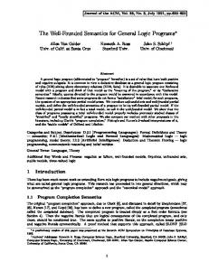
Fig. 5. Symbolic fixpoint computation for the program in Example 5 ourselves to considering LO programs (i.e., without the constant 1) it turns out that we need only consider constraints of the form x ≥ c, which can be abstracted away by considering the upward closure of b c, as we did in Section 5. The reader can note that the 4 relation defined above for constraints is an extension of the multiset inclusion relation we used in Section 5. The construction based on ⊑ can be directly incorporated into the semantic framework presented in Section 7, where, for the sake of simplicity, we have adopted an approach based on ⊆. Of course, relation ⊆ is stronger than ⊑, therefore a computation based on ⊑ is correct and it terminates every time a computation based on ⊆ does. However, the converse does not always hold, and this is why a concrete algorithm for computing the least fixpoint of SP1 relies on subsumption. Let us see an example. Example 5 We calculate the fixpoint semantics for the following LO1 program made up of six clauses: 1 · a ◦− 1 ........... 2 · a ............... b ◦− ⊤ ............... 3 · c ............. c ◦− ⊤ ........... 4 · b ................ b ◦− a 5 · a ◦− b 6 · c ◦− a & b Let Σ = {a, b, c} and consider constraints over the variables x = hxa , xb , xc i. We have that SP ↑0 = ∅ 1[xa = 0 ∧ xb = 0 ∧ xc = 0], therefore, by the first clause, ϕ ∈ SP ↑1 , where ϕ = ∃x′ ·(xa′ = 0∧xb′ = 0∧xc′ = 0∧xa = xa′ +1∧xb = xb′ ∧xc = xc′ ), which is equivalent to xa = 1 ∧ xb = 0 ∧ xc = 0. From now on, we leave to the reader the details concerning equivalence of constraints. By reasoning in a similar way, using clauses 2. and 3. we calculate SP ↑1 (see Figure 5). We now compute SP ↑2 . By 4., as SP ↑1 a[xa = 0 ∧ xb = 0 ∧ xc = 0], we get xa = 0 ∧ xb = 2 ∧ xc = 0, and, similarly, we get xa ≥ 0 ∧ xb ≥ 3 ∧ xc ≥ 0. By 5., we have xa ≥ 2 ∧ xb ≥ 0 ∧ xc ≥ 0, while clause 6. is not (yet) applicable. Therefore, modulo redundant constraints (i.e., constraints subsumed by the already calculated ones) the value of SP ↑2 is given in Figure 5.


27

Now, we can compute SP ↑3 . By 4. and xa ≥ 2 ∧ xb ≥ 0 ∧ xc ≥ 0 ∈ SP ↑2 we get xa ≥ 1 ∧ xb ≥ 2 ∧ xc ≥ 0, which is subsumed by xa ≥ 1 ∧ xb ≥ 1 ∧ xc ≥ 0. By 5. and xa = 0 ∧ xb = 2 ∧ xc = 0, we get xa = 1 ∧ xb = 1 ∧ xc = 0, subsumed by xa ≥ 1∧xb ≥ 1∧xc ≥ 0. Similarly, by 5. and xa ≥ 0∧xb ≥ 3∧xc ≥ 0 we get redundant information. By 6., from xa ≥ 1∧xb ≥ 1∧xc ≥ 0 and xa = 0∧xb = 2∧xc = 0 we get xa = 0 ∧ xb = 1 ∧ xc = 1, from xa ≥ 1 ∧ xb ≥ 1 ∧ xc ≥ 0 and xa ≥ 0 ∧ xb ≥ 3 ∧ xc ≥ 0 we get xa ≥ 0 ∧ xb ≥ 2 ∧ xc ≥ 1, and finally from xa ≥ 2 ∧ xb ≥ 0 ∧ xc ≥ 0 and xa ≥ 1 ∧ xb ≥ 1 ∧ xc ≥ 0 we have xa ≥ 1 ∧ xb ≥ 0 ∧ xc ≥ 1. The reader can verify that no additional provable multisets can be obtained. It is somewhat tedious, but in no way difficult, to verify that clause 6. yields only redundant information when applied to every possible couple of constraints in SP ↑3 . We have then SP ↑4 = SP ↑3 = SymbF1 (P ), so that in this particular case we achieve termination. We can reformulate the operational semantics of P using the more suggestive multiset notation (we recall that [[A]] = {B | A 4 B}, where 4 is multiset inclusion): F1 (P ) = {{a}, {b, b}, {b, c}} ∪ [[{a, b}, {c, c}, {b, b, b}, {a, a}, {b, b, c}, {a, c}]]· 2 It is often not the case that the symbolic computation of LO1 program semantics can be carried out in a finite number of steps. Nevertheless, it is important to remark that viewing the bottom-up evaluation of LO1 programs as a least fixpoint computation over infinite-state integer systems allows us to apply techniques and tools developed in infinite-state model checking (see e.g. (Abdulla et al., 1996; Bultan et al., 1997; Delzanno & Podelski, 1999; Finkel & Schnoebelen, 2001; Henzinger et al., 1997)) and program analysis (Cousot & Halbwachs, 1978) to compute approximations of the least fixpoint of SP1 . In the next section we will present an interesting application of the semantical framework we have presented so far. Namely, we shall make a detailed comparison between LO and Disjunctive Logic Programming. This will help us in clarifying the relations and the relative strength of the languages. After recalling the basic definitions of DLP in Section 9, we will present our view of DLP as an abstraction of LO in Section 10. Finally, in Section 11 we will give a few hints on how to employ this framework to study reachability problems in Petri Nets.

9 An Application of the Semantics: Relation with DLP As anticipated in the introduction, the paradigms of linear logic programming and Disjunctive Logic Programming have in common the use of multi-headed clauses. However, the operational interpretation of the extended notion of clause is quite different in the two paradigms. In fact, as shown in (Bozzano et al., 2000b), from a proof-theoretical perspective it is possible to view LO as a sub-structural fragment of DLP in which the rule of contraction is forbidden on the right-hand side of sequents. While proof theory allows one to compare the top-down semantics of the two languages, abstract interpretation (Cousot & Cousot, 1977) can be used to relate

28


the fixpoint, bottom-up evaluation of programs. In the following we will focus on the latter approach, exploiting our semantics of LO and the bottom-up semantics of DLP given in (Minker et al., 1991). For the sake of clarity, we will use superscripts in order to distinguish between the fixpoint operators for LO and DLP, which will be denoted by TPlo and TPdlp , respectively. First of all, we recall some definitions concerning Disjunctive Logic Programming. A disjunctive logic program as defined in (Minker et al., 1991) is a finite set of clauses A1 ∨ . . . ∨ An ← B1 ∧ . . . ∧ Bm , where n ≥ 1, m ≥ 0, and Ai and Bi are atomic formulas. A disjunctive goal is of the form ← C1 , . . . , Cn , where Ci is a positive clause (i.e., a disjunction of atomic formulas) for i : 1, . . . , n. To make the language symmetric, in this paper we will consider extended clauses of the form A1 ∨ . . . ∨ An ← C1 ∧ . . . ∧ Cm containing positive clauses in the body. Following (Minker et al., 1991), we will identify positive clauses with sets of atoms. In order to define the operational and denotational semantics of DLP, we need the following notions. Definition 9.1 (Disjunctive Herbrand Base) The disjunctive Herbrand base of a program P , for short DHBP , is the set of all positive clauses formed by an arbitrary number of atoms. Definition 9.2 (Disjunctive Interpretation) A subset I of the disjunctive Herbrand base DHBP is called a disjunctive Herbrand interpretation. Definition 9.3 (Ground SLO-derivation) Let P be a DLP program. An SLO-derivation of a ground goal G from P consists of a sequence of goals G0 = G, G1 , . . . such that for all i ≥ 0, Gi+1 is obtained from Gi =← (C1 , . . . , Cm , . . . , Ck ) as follows: - C ← D1 ∧ . . . ∧ Dq is a ground instance of a clause in P such that C is contained in Cm (the selected clause); - Gi+1 is the goal ← (C1 , . . . , Cm−1 , D1 ∨ Cm , . . . , Dq ∨ Cm , Cm+1 , . . . , Ck ). Definition 9.4 (SLO-refutation) Let P be a DLP program. An SLO-refutation of a ground goal G from P is an SLO-derivation G0 , G1 , . . . , Gk s.t. Gk consists of the empty clause only. As SLD-resolution for Horn programs, SLO-resolution gives us a procedural interpretation of DLP programs. The operational semantics is defined then as follows: OPdlp = {C | C ∈ DHBP , ← C has an SLO-refutation}· As for Horn programs, it is possible to define a fixpoint semantics via the following operator (where gnd(P ) denotes the set of ground instances of clauses in P ).


29

Definition 9.5 (The TPdlp Operator ) Given a DLP program P and I ⊆ DHBP , TPdlp (I )

= { C ∈ DHBP | C ′ ← D1 , . . . , Dn ∈ gnd(P ), Di ∨ Ci ∈ I , i : 1, . . . , n C = C ′ ∨ C1 ∨ . . . ∨ Cn }·

The operator TPdlp is monotonic and continuous on the lattice of interpretations ordered w.r.t. set inclusion. Based on this property, the fixpoint semantics is defined as FPdlp = lf p(TPdlp ) = TPdlp ↑ω . As shown in (Minker et al., 1991), for all C ∈ OPdlp there exists C ′ ∈ FPdlp s.t. C ′ implies C . Note that for two ground clauses C and C ′ , C implies C ′ if and only if C ⊆ C ′ . This suggests that interpretations can also be ordered w.r.t. subset inclusion for their elements, i.e., I ⊑ J if and only if for all A ∈ I there exists B ∈ J such that B ⊆ A (B implies A). In the rest of the paper we will consider this latter ordering. Example 6 Consider the disjunctive program P = {r (a), p(X ) ∨ q(X ) ← r (X )} and the auxiliary predicate t . Then, DHBP = {r (a), p(a), q(a), t (a), p(a) ∨ r (a), p(a) ∨ q(a), p(a) ∨ q(a) ∨ r (a), . . .}. Furthermore, the goal G0 =← (p(a) ∨ q(a) ∨ t (a)) has the refutation G0 , G1 =← (p(a) ∨ q(a) ∨ t (a) ∨ r (a)), G2 where G2 consists of the empty clause only. The fixpoint semantics of P is as follows FPdlp = {r (a), p(a) ∨ q(a)}. Note that p(a) ∨ q(a) ∨ t (a) is implied by p(a) ∨ q(a). 2 We note that the definition of the TPdlp operator can be re-formulated in such a way that its input and output domains contain multisets instead of sets of atoms (i.e., we can consider interpretations which are sets of multisets of atoms). In fact, we can always map a multiset to its underlying set, i.e., the set containing the elements with multiplicity greater than zero, and, vice versa, a set can be viewed as a multiset in which each element has multiplicity equal to one. In the following we will assume that TPdlp is defined on domains containing multisets. As the fixpoint operator for LO is defined on the same kind of domains, this will make the comparison between the two operators easier. Furthermore, without loss of generality, we will make the assumption that in clauses like A1 ∨ . . . ∨ An ← C1 ∧ . . . ∧ Cm , the Ai ’s are all distinct and each Cj consist of distinct atoms. This will simplify the embedding of DLP clauses into linear logic. The previous definitions can be easily adapted. Now, we give a closer look at the formal presentations of DLP and LO. As said in the Introduction, we only need to consider a fragment of LO in which connectives can not be arbitrarily nested in goals, like in DLP. This fragment can be described by the following grammar: H ::= A1

................ ......... ...

...

................ ......... ...

An

D ::= H ◦− G | D & D G ::= H1 & . . . & Hn | ⊤ where Ai is an atomic formula. The comparison between the two languages is based on the idea that, to some extent, linear connectives, i.e., additive conjunction

30

M. Bozzano, G. Delzanno and M. Martelli ............

& and multiplicative disjunction ..............., should behave like classical conjunction ∧ and classical disjunction ∨. Actually, classical connectives give rise to a fixpoint semantics for DLP which is a proper abstraction of the semantics for LO. The translation between linear and classical connectives is given via the following mapping ⌈·⌉: ⌈F ∨ G⌉ = ⌈F ⌉

.............. .......... ...

⌈G⌉, ⌈F ∧ G⌉ = ⌈F ⌉ & ⌈G⌉, ⌈F ← G⌉ = ⌈F ⌉ ◦− ⌈G⌉, ⌈tt⌉ = ⊤·

In order to make the comparison between DLP and LO more direct, it is possible to present DLP by means of the following grammar: H ::= A1 ∨ . . . ∨ An D ::= H ← G | D ∧ D G ::= H1 ∧ . . . ∧ Hn

| tt

where Ai is an atomic formula. A DLP program P is now a D-clause, whereas DLP goals are represented (modulo ‘←’) as G-formulas. Here, we have introduced an explicit constant tt for true and we have written unit clauses (i.e., with empty body) with the syntax A1 ∨ . . . ∨ An ← tt. With these conventions, the grammars for LO and DLP given above are exactly the same modulo the translation ⌈·⌉. The definitions concerning the operational and fixpoint semantics for DLP given previously can be adapted in a straightforward manner. The reader can also note that by definition of DLP program, the image of ⌈·⌉ returns a class of LO programs where both the head and the disjuncts in the body have no repeated occurrences of the same atom. We conclude this section by specializing our fixpoint semantics for LO, given in Section 5, to the simpler fragment presented above. We give the following definition for the TPlo operator: Definition 9.6 (TPlo operator ) Given an LO program P and an interpretation I , the operator TPlo is defined as follows: TPlo (I )

=

b + (C1 • . . . • Cn ) | H ◦− D1 & . . . & Dn ∈ P , ∀i = 1, . . . , n, D ci + Ci ∈ I } {H b | H ◦− ⊤ ∈ P } ∪ {H

The operator TPlo is monotonic and continuous over the lattice of Herbrand interpretations (ordered w.r.t. ⊑). Thus, the fixpoint semantics of an LO-program P is defined as ω G TPlo ↑i · FPlo = i=0

A completeness result similar to that of Section 5, stating the equivalence between the operational and fixpoint semantics, obviously holds for the fragment of LO considered here. 10 DLP as Abstraction of LO The fixpoint semantics of LO allows us to investigate in more depth the relationships between LO and DLP. For this purpose, we can employ the mathematical tools


31

provided by abstract interpretation (Cousot & Cousot, 1977), and in particular the notion of completeness (Cousot & Cousot, 1977; Giacobazzi & Ranzato, 1997) that qualifies the precision of an abstraction. Informally, the comparison between LO and DLP fixpoint semantics is based on the abstraction that maps multisets into sets of atomic formulas (positive clauses). This abstraction induces a Galois connection between the semantic domains of DLP and LO. We prove that the fixpoint semantics of the translation of an LO program in DLP is a correct abstraction of the fixpoint semantics of the original LO program. Furthermore, we show that this abstraction is not fully complete with respect to LO semantics. In a fully complete abstraction the result of interleaving the application of the abstract fixpoint operator with the abstraction α coincides with the abstraction of the concrete fixpoint operator. For a complete abstraction, a similar relation holds for fixpoints, i.e., the fixpoint of the abstract operator coincides with the abstraction of the fixpoint of the concrete one. We isolate an interesting class of LO programs for which we show that the property of completeness holds. In particular, completeness holds if we forbid conjunctions in the body of clauses. The resulting class of LO programs is still very interesting, as it can be used to encode Petri Nets. Abstract Interpretation (Cousot & Cousot, 1977; Cousot & Cousot, 1979) is a classical framework for semantics approximation which is used for the construction of semantics-based program analysis algorithms. Given a semantics and an abstraction of the language constructors and standard data, abstract interpretation determines an abstract representation of the language which is, by construction, sound with respect to the standard semantics. This new representation enables the calculation of the abstract semantics in finite time, although it implies some loss of precision. We recall here some key concepts in abstract interpretation, which the reader can find in (Cousot & Cousot, 1977; Cousot & Cousot, 1979; Giacobazzi & Ranzato, 1997). Given a concrete semantics hC , TP i, specified by a concrete domain (complete lattice) C and a (monotone) fixpoint operator TP : C → C , the abstract semantics can be specified by an abstract domain A and an abstract fixpoint operator TP# . In this context, program semantics is given by lf p(TP ), and its abstraction is lf p(TP# ). The concrete and abstract semantics S = hC , TP i and S # = hA, TP# i are related by a Galois connection hα, C , A, γi, where α : C → A and γ : A → C are called abstraction and concretization functions, respectively. S # is called a sound abstraction of S if for all P , α(lf p(TP )) ≤A lf p(TP# ). This condition is implied by the strongest property of full soundness, which requires that α ◦ TP ≤A TP# ◦ α. The notions of completeness and full completeness are dual with respect to those of soundness. Namely, S # is a (fully) complete abstraction of S if for all P , (TP# ◦ α ≤A α ◦ TP ) lf p(TP# ) ≤A α(lf p(TP )). Often, the notion of completeness is assumed to include soundness (i.e., we impose ’=’ in the previous equations). It is well-known (Cousot & Cousot, 1979) that the abstract domain A induces a best correct approximation of TP , which is given by α ◦ TP ◦ γ, and that it is possible to define a (fully) complete abstract operator TP# if and only if the best correct approximation is (fully) complete. It can be proved that for a fixed concrete semantics, (full) completeness of an abstract interpretation only

32


depends on the choice of the abstract domain. The problem of achieving a (fully) complete abstract interpretation starting from a correct one, by either refining or simplifying the abstract domain, is studied in (Giacobazzi & Ranzato, 1997). We conclude by observing that an equivalent presentation of abstract interpretation is based on closure operators (Cousot & Cousot, 1979), i.e. functions from a concrete domain C to itself which are monotone, idempotent and extensive. This approach provides independence from specific representations of abstract domain’s objects (the abstract domain is given by the image, i.e., the set of fixpoints, of the closure operator). We are now in the position of connecting the LO (concrete) semantics with the DLP (abstract) semantics. We define the abstract interpretation as a closure operator on the lattice I, the domain of LO interpretations of Definition 5.1. In fact, as mentioned before, we can consider disjunctive interpretations as a subclass of I (i.e., all sets in I). We recall that in I the ordering of interpretations is defined as follows: I ⊑ J iff for all B ∈ I there exists A ∈ J such that A is a sub-multiset of B (i.e., for disjunctive interpretations, A ⊆ B ). We give the following definitions. Definition 10.1 (Abstract Interpretation from LO to DLP ) The abstract interpretation is defined by the closure operator α : I → I such that for every I ∈ I, α(I ) = {α(A) | A ∈ I}, where for a given multiset A, α(A) is the multiset such that for every i = 1, . . . , n, Occα(A) (ai ) = 0 if OccA (ai ) = 0, Occα(A) (ai ) = 1 otherwise (i.e., we abstract a multiset with the corresponding set). Definition 10.2 (Abstract semantics) The abstract fixpoint semantics is given by lf p(TP# ), where the abstract fixpoint operator TP# is defined as (α ◦ TPlo ). According to (Cousot & Cousot, 1979), α ◦ TPlo is the best correct approximation of the concrete fixpoint operator TPlo , for the fixed abstraction α. The abstraction α, as said before, transforms multisets into sets by forgetting multiple occurrences of atoms. It is not difficult to convince ourselves that TP# is indeed the TPdlp operator for disjunctive logic programs, provided that, as discussed in Section 9, we consider TPdlp defined over domains containing multisets instead of sets (actually, we are identifying TPdlp input domain with the abstract domain which is given by the set of fixpoints, i.e., the image, of the closure operator α). The operations • (least upper bound of multisets) and + (multiset union) used in the definition of TPlo are interchangeable (because of the subsequent application of the operator α) and correspond to set (multiset) union in the definition of TPdlp . We have the following results. Proposition 10 (DLP is an abstraction of LO ) For every DLP program P and disjunctive (hence LO) interpretation I , TPdlp (I ) = # T⌈P ⌉ (I ). Proof By definitions.


33

Proposition 11 (DLP is a correct abstraction of LO ) For every LO program P , the abstract semantics is a fully sound abstraction of the concrete semantics, that is, for every interpretation I , α(TPlo (I )) ⊑ TP# (α(I ))· Proof As TP# = α ◦ TPlo and I ⊑ α(I ), the proposition follows by monotonicity of TP# . The previous result implies soundness, i.e. α(lf p(TPlo )) ⊑ lf p(TP# ). The strong property of full completeness does not hold for the abstraction. To see why, take as a counterexample the single clause a ◦− b and the interpretation I with the single multiset {b, b}. Then, α(TPlo (I )) = {{a, b}}, TP# (α(I )) = {{a}}, and TP# (α(I )) 6⊑ α(TPlo (I )). We conclude this section showing that the abstraction is complete for the subclass of LO programs whose clauses contain at most one conjunct in the body. We will address some applications of this result in Section 11. (Note: the abstraction not being fully complete has a counterpart in the fact that in general h > 1 in the following lemma, i.e., more than one step of TPlo is necessary to simulate one step of TP# ).) Lemma 5 Let P be an LO program in which every clause has at most one conjunct in the body (i.e., conjunction is forbidden), and I , J two interpretations. If I ⊑ α(J ) then there exists a natural number h such that α(TPlo (I )) ⊑ α(TPlo ↑h (J )). Proof Suppose I ⊑ α(J ) and A ∈ α(TPlo (I )). Then there exists A′ ∈ TPlo (I ) s.t. A = α(A′ ). By definition of TPlo , there exists a clause H ◦− D ∈ P (the case for unit b + C ∈ I and A′ = H b + C. As I ⊑ α(J ), we also have clauses is trivial) s.t. D b b + C = α(K). Let D + C ∈ α(J ), which implies that there exists K ∈ J s.t. D n b p = min{n | K 4 (D + C) } (it is immediate to prove that such a p exists), and b + C)p . We have that K 4 M, therefore M ∈ J (because K ∈ J and let M = (D b + (C + (D b + C)p−1 ) ∈ J , and, by definition J is upward-closed). Now, M = D lo p−1 b b of TP (H ◦− D ∈ P ), H + C + (D + C) ∈ TPlo (J ). By repeatedly applying lo b + C)p ∈ T lo ↑p (J ). Therefore TP (the proof is by induction on p) we get (H P p lo b + C) = α((H b + C) ) ∈ α(T ↑p (J )). A = α(H P Proposition 12 Let P be an LO program in which every clause has at most one conjunct in the body. Then α(lf p(TPlo )) = lf p(TP# ). Proof By a simple induction, using Lemma 5, we have that for every k there exists h s.t. TP#↑k ⊑ α(TPlo ↑h ). Therefore lf p(TP# ) ⊑ α(lf p(TPlo )). The class of LO programs with one conjunct in the body is still very interesting. Below, we show how this result could be exploited to study reachability problems in Petri Nets.

34

M. Bozzano, G. Delzanno and M. Martelli 11 Other Applications: Relation with Petri Nets

As shown in the proof of Proposition 6, the class of propositional LO programs with one conjunct in the body is equivalent to VAS, i.e., to Petri Nets. Intuitively, a multiset rewriting rule can be used to describe the effect of firing a Petri Net ........... .......... ........... transition. For instance, the clause a ................. b ................. b ◦− c ................. c can be interpreted as the Petri Net transition that removes one token from place a, two tokens from place b, and adds two tokens to place c. As a consequence, a (possibly infinite) execution (sequence of goals G0 , G1 , . . .) of a restricted LO program denotes an execution of the corresponding Petri Net. The initial goal G0 can be viewed as the initial marking of the Petri Net. Consider now the fact F ≡ c ◦− ⊤, and let G0 be the ............ ........... goal a ................ a ................ b. Then, the sequent P ∪ F ⇒ G0 is provable in LO if and only if there exists a reachable marking having at least one token in place c. In other words, the fact F can be used to implicitly represent an infinite set of markings (its upward closure) of the corresponding Petri Net. Our bottom-up semantics can be use to effectively compute the set Pre ∗ (F ) (using the terminology of (Abdulla et al., 1996)) of markings that can reach a marking in the denotation of F . This idea can be used to verify safety properties of concurrent systems. A safety property S can be viewed as a set of good states (markings) of a given concurrent system (Petri Net). The system satisfies the property if the set of states that are reachable from the initial state G0 are all contained in S . Symmetrically, the set ¬S represents the set of bad states. Thus, the systems can be proved correct by showing that Pre ∗ (¬S ) does not contain the initial state G0 , i.e., by applying the bottom-up algorithm starting from a fact denoting ¬S . It is interesting to note that in many real examples ¬S is indeed an upward closed set of states (e.g. the set of states where there are at least two processes in the critical section are the the typical bad states of a mutual exclusion algorithm). In general, the complexity of computing Pre ∗ (F ), for some F , can be very high. However, the results of Section 10 show that the fixpoint semantics of DLP can be used to approximate the set Pre ∗ (F ). Completeness implies that all properties that are preserved by the abstraction can be checked equivalently over the concrete and the abstract domain. In our setting the kind of properties that satisfy this requirement can be informally characterized as ‘at least one’-properties (e.g. is there at least one token in place P in a reachable marking?). This kind of properties can be used to check ‘mutual exclusion’ for a concurrent system represented via a Petri Net. Suppose we want to prove that a system ensures mutual exclusion for two processes represented via a Petri Net. Process pi is in the critical section whenever a token is in a special place csi for i : 1, 2. Violations of mutual exclusion are expressed as the set of states with at least one token in place cs1 and one token in state cs2 . Thus, the fixpoint semantics of the DLP program obtained as translation of the Petri Net (LO program) union the fact cs1 ∨ cs2 is an abstraction of the set of backward reachable states. We obtain a full-test for mutual exclusion properties, whenever the initial states can be expressed again as at least one properties (i.e., whenever membership of the initial states in the set of abstract reachable states can be determined exactly).


35

12 Related Works Our work is inspired to the general decidability results for infinite-state systems based on the theory of well-quasi orderings given in (Abdulla et al., 1996; Finkel & Schnoebelen, 2001). In fact, the construction of the least fixpoint of SP and SP1 can be viewed as an instance of the backward reachability algorithm for transition systems presented in (Abdulla et al., 1996). Differently from (Abdulla et al., 1996; Finkel & Schnoebelen, 2001), we need to add special rules (via the satisfiability relation ) to handle formulas with the connectives & , ⊤ and 1. Other sources of inspiration come from linear logic programming. In (Harland & Winikoff, 1998), the authors present an abstract deductive system for the bottomup evaluation of linear logic programs. The left introduction rules plus weakening and cut are used to compute the logical consequences of a given formula. The satisfiability relations we use in the definition of the fixpoint operators correspond to top-down steps within their bottom-up evaluation scheme. The framework is given for a more general fragment than LO. However, they do not provide an effective fixpoint operator as we did in the case of LO and LO1 , and they do not discuss computability issues for the resulting derivability relation. In (Andreoli et al., 1997), Andreoli, Pareschi and Castagnetti present a partial evaluation scheme for propositional LO (i.e without 1). Given an initial goal G, they use a construction similar to Karp and Miller’s coverability tree (Karp & Miller, 1969) for Petri Nets to build a finite representation of a proof tree for G. During the top-down construction of the graph for G, they apply in fact a generalization step that works as follows. If a goal, say B, that has to be proved is subsumed by a node already visited, say A, (i.e., B = A + A′ ), then the part of proof tree between the two goals is replaced by a proof tree for A + (A′ )∗ ; A + (A′ )∗ is a finite representation of the union of A with the closure of A′ . They use Dickson’s Lemma to show that the construction always terminates. In the case of LO, the main difference with our approach is that we give a goal independent bottom-up algorithm. Technically, another difference is that in our fixpoint semantics we do not need any generalization step. In fact, in our setting the computation starts directly from (a representation of) upward-closed sets of contexts. This simplifies the computation as shown in Example 3 (we only need to test 4). Finally, differently from (Andreoli et al., 1997), in this paper we have given also a formal semantics for the extension of LO with the constant 1. The partial evaluation scheme of (Andreoli et al., 1997) is aimed at compile-time optimizations of abstractions of LinLog programs. Another example of analysis of concurrent languages based on linear logic is given in (Kobayashi et al., 1995), where the authors present a type inference procedure that returns an approximation of the number of messages exchanged by HACL processes. In (Cervesato, 1995) Cervesato shows how to encode Petri Nets in LO, Lolli and Forum by exploiting the different features of these languages. We used some of these ideas to prove Proposition 6. Finally, we have discussed the similarities between our semantics and the bottomup semantics for Disjunctive Logic Programming of Minker, Rajasekar and Lobo

36


(Minker et al., 1991). In a disjunctive logic program, the head of a clause is a disjunction of atomic formulas, whereas the body is a conjunction of atomic formulas. In the semantics of (Minker et al., 1991) interpretations are collections of sets (disjunctions) of atomic formulas. Only minimal (w.r.t. set inclusion) sets are kept at each fixpoint iteration. In contrast, in our setting we need to consider collections of multisets of formulas. Therefore, in the propositional case in order to prove the convergence of the fixpoint iteration, we need an argument (Dickson’s lemma) stronger than the finiteness of the extended Herbrand base of (Minker et al., 1991) (collection of all minimal sets).

13 Conclusions and Future Work In this paper we have defined a bottom-up semantics for the fragment of LinLog (Andreoli, 1992) consisting of the language LO (Andreoli & Pareschi, 1991) enriched with the constant 1. In the propositional case, we have shown that without 1 the fixpoint semantics is finitely computable. Our fixpoint operator is defined over constraints and gives us an effective way to evaluate bottom-up (abstractions of) linear logic programs. To conclude, let us discuss the directions of research that we find more promising. Linear Logic Programming. It would be interesting to extend the techniques we presented in this paper to larger fragments of linear logic. In particular, it would be interesting to define a bottom-up evaluation for languages like Lolli (Hodas & Miller, 1994) and Lygon (Harland & Pym, 1994), and to study techniques for firstorder formulation for all these languages. An extension of the present framework to the first-order case should also take into account the so-called S-semantics (Falaschi et al., 1993; Bossi et al., 1994), in order to model observables like computed answer substitutions and to cope with issues like compositional semantics. Concerning LO, we would also like to look at the connection with the so-called Chemical Abstract Machine metaphor (Andreoli et al., 1993). Verification. In (Delzanno & Podelski, 1999), the authors show that properties of concurrent systems expressed in temporal logic can be defined in terms of fixpoint semantics of a logic program that encodes the transition system of a concurrent system. In (Delzanno & Podelski, 1999), synchronization between processes is achieved via shared variables, whereas in linear logic synchronization can be expressed via multiple headed clauses. Thus, our semantics might be a first step towards the extension of the metaphor of (Delzanno & Podelski, 1999) to concurrent systems in which synchronization is expressed at the logical level (see Section 11). The other way round, through the connection between semantics and verification, techniques used for infinite-state systems with integer variables (see e.g. (Delzanno & Podelski, 1999; Bultan et al., 1997; Henzinger et al., 1997)) can be re-used in order to compute a static analysis of linear logic programs. Proof Theory. The connection we establish in this paper indicates a potential connection between the general decidability results for infinite-state systems of (Abdulla et al., 1996; Finkel & Schnoebelen, 2001) and provability in sub-structural


37

logics like LO and affine linear logic (Kopylov, 1995). Viewing the provability relation as a transition relation, it might be possible to find a notion of well-structured proof system (paraphrasing the notion of well-structured transition systems of (Abdulla et al., 1996; Finkel & Schnoebelen, 2001)), i.e., a general notion of provability that ensures the termination of the bottom-up generation of valid formulas. Relations between DLP and LO. We hope that our study will give rise to new ideas for the analysis of LO programs. As an example, it could be interesting to study weak notions of negation for LO that are based on the negation of DLP. Moreover, we can use DLP operational and fixpoint semantics to analyze Petri Nets, given that the abstraction is complete in this case. Finally, there are still some open questions concerning the relation between DLP and LO in the setting of abstract interpretation. In particular, we would like to study the notion of completeness for the general class of LO programs (we remark that the example in (Bozzano et al., 2000b) showing incompleteness was wrong). We would also like to analyze in more detail the connection between the notion of (full) completeness of the abstraction and proof-theoretic properties of provability in sub-structural logics, which has been only partly addressed in (Bozzano et al., 2000b).

Acknowledgments The authors would like to thank Maurizio Gabbrielli for his support, Jean-Marc Andreoli for useful comments on the use of LO, and the anonymous reviewers for providing us suggestions and references that helped us to improve the presentation of the paper.

References Abdulla, P. A., Cer¯ ans, K., Jonsson, B., & Tsay, Y.-K. (1996). General Decidability Theorems for Infinite-State Systems. Pages 313–321 of: Proc. 11th Annual IEEE Int. Symposium on Logic in Computer Science (LICS’96). IEEE Computer Society Press. Andreoli, J.-M. (1992). Logic Programming with Focusing Proofs in Linear Logic. Journal of Logic and Computation, 2(3), 297–347. Andreoli, J.-M. (1996). Coordination in LO. Pages 42–64 of: Andreoli, J.-M., Hankin, C., & Metayer, D. Le (eds), Coordination Programming: Mechanisms, Models and Semantics. Imperial College Press. Andreoli, J.-M., & Pareschi, R. (1991). Linear Objects: Logical Processes with Built-In Inheritance. New Generation Computing, 9(3-4), 445–473. Andreoli, J.-M., Leth, L., Pareschi, R., & Thomsen, B. (1993). True Concurrency Semantics for a Linear Logic Programming Language with Broadcast Communication. Pages 182–198 of: Gaudel, M.-C., & Jouannaud, J.-P. (eds), Proc. Theory and Practice of Software Development, International Joint Conference CAAP/FASE (TAPSOFT’93). Lecture Notes in Computer Science, vol. 668. Springer-Verlag. Andreoli, J.-M., Pareschi, R., & Castagnetti, T. (1997). Static Analysis of Linear Logic Programming. New Generation Computing, 15(4), 449–481. Bossi, A., Gabbrielli, M., Levi, G., & Martelli, M. (1994). The s-Semantics Approach: Theory and Applications. Journal of logic programming, 19-20, 149–197.

38


Bozzano, M., Delzanno, G., & Martelli, M. (2000a). A Bottom-up Semantics for Linear Logic Programs. Pages 92–102 of: Gabbrielli, M., & Pfenning, F. (eds), Proc. 2nd International Conference on Principles and Practice of Declarative Programming (PPDP’00). ACM Press. Bozzano, M., Delzanno, G., & Martelli, M. (2000b). DLP as an Abstraction of LO. On the relations between Disjunctive and Linear Logic Programming. Presented at 2000 Joint Conference on Declarative programming (APPIA-GULP-PRODE’00). Available from URL http://nutella.di.unipi.it/∼agp00/AccptAbstr.html. Bultan, T., Gerber, R., & Pugh, W. (1997). Symbolic Model Checking of Infinite State Systems Using Presburger Arithmetics. Pages 400–411 of: O. Grumberg (ed), Proc. 9th International Conference on Computer Aided Verification (CAV’97). Lecture Notes in Computer Science, vol. 1254. Springer-Verlag. Cervesato, I. (1995). Petri Nets and Linear Logic: a Case Study for Logic Programming. Pages 313–318 of: M. Alpuente and M. I. Sessa (ed), Proc. 1995 Joint Conference on Declarative Programming (GULP-PRODE’95). Palladio Press. Cousot, P., & Cousot, R. (1977). Abstract Interpretation: A Unified Lattice Model for Static Analysis of Programs by Construction or Approximation of Fix-Points. Pages 238–252 of: Proc. 4th Symposium on Principles of Programming Languages (POPL’77). ACM Press. Cousot, P., & Cousot, R. (1979). Systematic Design of Program Analysis Frameworks. Pages 269–282 of: Proc. 6th Symposium on Principles of Programming Languages (POPL’79). ACM Press. Cousot, P., & Halbwachs, N. (1978). Automatic Discovery of Linear Restraints Among Variables of a Program. Pages 84–96 of: Proc. 5th Symposium on Principles of Programming Languages (POPL’78). ACM Press. Delzanno, G., & Podelski, A. (1999). Model checking in CLP. Pages 223–239 of: Cleaveland, R. (ed), Proc. 5th International Conference on Tools and Algorithms for Construction and Analysis of Systems (TACAS’99). Lecture Notes in Computer Science, vol. 1579. Springer-Verlag. Dickson, L. E. (1913). Finiteness of the Odd Perfect and Primitive Abundant Numbers with n Distinct Prime Factors. American Journal of Mathematics, 35(413-422). Esparza, J., & Nielsen, M. (1994). Decidability Issues for Petri Nets - a Survey. Journal of Informatik Processing and Cybernetics, 30(3), 143–160. Falaschi, M., Levi, G., Martelli, M., & Palamidessi, C. (1993). A Model-Theoretic Reconstruction of the Operational Semantics of Logic Programs. Information and Computation, 103(1), 86–113. Finkel, A., & Schnoebelen, P. (2001). Well-Structured Transition Systems Everywhere! Theoretical Computer Science, 256(1-2), 63–92. Gabbrielli, M., Dore, M. G., & Levi, G. (1995). Observable semantics for Constraint Logic Programs. Journal of Logic and Computation, 5(2), 133–171. Giacobazzi, R., & Ranzato, F. (1997). Completeness in Abstract Interpretation: A Domain Perspective. Pages 231–245 of: M. Johnson (ed), Proc. 6th International Conference on Algebraic Methodology and Software Technology (AMAST’97). Lecture Notes in Computer Science, vol. 1349. Springer-Verlag. Girard, J.Y. (1987). Linear logic. Theoretical computer science, 50:1, 1–102. Harland, J., & Pym, D. J. (1994). A Uniform Proof-Theoretic Investigation of Linear Logic Programming. Journal of Logic and Computation, 4(2), 175–207. Harland, J., & Winikoff, M. (1998). Making Logic Programs Reactive. Pages 43–58 of: Proc. JICSLP’98 Workshop on Transactions and Change in Logic Databases (Dynamics’98).


39

Henzinger, T. A., Ho, P.-H., & Wong-Toi, H. (1997). HYTECH: A Model Checker for Hybrid Systems. Pages 460–463 of: Grumberg, O. (ed), Proc. 9th International Conference on Computer Aided Verification (CAV’97). Lecture Notes in Computer Science, vol. 1254. Springer-Verlag. Hodas, J., & Miller, D. (1994). Logic Programming in a Fragment of Intuitionistic Linear Logic. Information and Computation, 110(2), 327–365. Jaffar, J., & Maher, M. J. (1994). Constraint Logic Programming: A survey. Journal of Logic Programming, 19-20, 503–581. Karp, R. M., & Miller, R. E. (1969). Parallel Program Schemata. Journal of Computer and System Sciences, 3(2), 147–195. Kobayashi, N., & Yonezawa, A. (1995). Asynchronous Communication Model based on Linear Logic. Formal Aspects of Computing, 7(2), 113–149. Kobayashi, N., Nakade, M., & Yonezawa, A. (1995). Static Analysis of Communication for Asynchronous Concurrent Programming Languages. Pages 225–242 of: Mycroft, A. (ed), Proc. 2th International Symposium on Static Analysis (SAS’95). Lecture Notes in Computer Science, vol. 983. Springer-Verlag. Kopylov, A. .P. (1995). Decidability of Linear Affine Logic. Pages 496–504 of: Kozen, D. (ed), Proc. 10th Annual IEEE Symposium on Logic in Computer Science (LICS’95). IEEE Computer Society Press. Lloyd, J. .W. (1987). Foundations of Logic Programming. Springer-Verlag. Miller, D. (1995). A Survey of Linear Logic Programming. Computational Logic: The Newsletter of the European Network of Excellence in Computational Logic, 2(2), 63– 67. Miller, D. (1996). Forum: A Multiple-Conclusion Specification Logic. Theoretical computer science, 165(1), 201–232. Minker, J., Rajasekar, A., & Lobo, J. (1991). Theory of Disjunctive Logic Programs. Pages 613–639 of: Lassez, J.L., & Plotkin, G. (eds), Computational Logic. Essays in Honor of Alan Robinson. MIT Press.