AN EFFECTIVE, SIMPLE TEMPO ESTIMATION METHOD BASED ON ...

AN EFFECTIVE, SIMPLE TEMPO ESTIMATION METHOD BASED ON SELF-SIMILARITY AND REGULARITY G. Tzanetakis, G. Percival [email protected], [email protected] Department of Computer Science University of Victoria, Canada ABSTRACT Tempo estimation is a fundamental problem in music information retrieval. It also forms the basis of other types of rhythmic analysis such as beat tracking and pattern detection. There is a large body of work in tempo estimation using a variety of different approaches that differ in their accuracy as well as their complexity. Fundamentally they take advantage of two properties of musical rhythm: 1) the music signal tends to be self-similar at periodicities related to the underlying rhythmic structure, 2) rhythmic events tend to be spaced regularly in time. We propose an algorithm for tempo estimation that is based on these two properties. We have tried to reduce the number of steps, parameters and modeling assumptions while retaining good performance and causality. The proposed approach outperforms a large number of existing tempo estimation methods and has similar performance to the best-performing ones. We believe that we have conducted the most comprehensive evaluation to date of tempo induction algorithms in terms of number of datasets and tracks. Index Terms— music information retrieval, tempo induction, rhythm analysis, audio signal processing 1. INTRODUCTION The automatic analysis of rhythm from audio signals is part of a number of music information retrieval (MIR) applications such as music similarity and recommendation, semi-automatic audio editing, automatic accompaniment, polyphonic transcription, beatsynchronous audio effects and computer assisted DJ systems. The two main tasks related to automatic analysis of rhythm that have been explored are tempo induction/estimation and beat tracking. The goal of tempo estimation is to automatically estimate the rate of musical beats in time. Beats can be defined as the locations in time where a human would “tap” their foot while listening to a piece of music. Beat tracking is the task of determining the locations of these beats in time, and is considerably harder in music in which the tempo varies over time [?]. In this paper, we focus solely on the task of tempo induction. Algorithms for tempo induction have become, over time, increasingly more complicated. They frequently contain multiple stages, each with many parameters which need to be adjusted. This complexity makes them less efficient, harder to optimize due to the large number of parameters, and difficult to replicate. Our goal has been to simplify the process by reducing the number of steps and parameters without affecting the accuracy of the algorithm. An additional motivation is that tempo induction is a task that most human listeners (even without musical training) can do reasonably well. Therefore, it should be possible to model this task without requiring complex models of musical knowledge.

After an early period in which systems were evaluated individually on small private datasets, since 2004 there have been three public datasets that have been frequently used to compare different approaches. We have conducted a thorough experimental investigation of multiple tempo induction algorithms which uses two datasets in addition to the usual three. We show that our proposed method demonstrates state-of-the-art performance that is statistically very close to the best performing systems we evaluated. The code of our algorithm, as well as the scripts used for the experimental comparison of all the different systems that were considered, is available as open source software. Moreover, all the datasets used are publicly available. By supporting reproducible digital signal processing research we hope to stimulate further experimentation in tempo estimation and automatic rhythmic analysis in general. The origins of work in tempo estimation and beat tracking can be traced to research in music psychology. There are some indications that humans solve these two problems separately. In the early (1973) two-level timing model proposed by Wing and Kristofferson [?], separate mechanisms for estimating the period (tempo) and phase (beat locations) are proposed by examining data from tapping a Morse key. A recent overview article of the tapping literature [?] summarizes the evidence for a two-process model that consists of a slow process which measures the underlying tempo and a fast synchronization process which measures the phase. Work in beat tracking started in the 1980s but mostly utilized symbolic input, frequently in the form of MIDI (Musical Instrument Digital Interface) signals. In the 1990s the first papers investigating beat tracking of audio signals appeared. A real-time beat tracking system based on a multiple agent architecture was proposed in 1994 [?]. Another influential early paper described a method that utilized comb filters to extract beats from polyphonic music [?]. There has been an increasing amount of interest in tempo induction for audio signals in recent years. A large experimental comparison of various tempo induction algorithms was conducted in 2004 as part of the International Conference on Music Information Retrieval (ISMIR) and presented in [?]. A more recent experimental comparison of 23 algorithms was performed in 2011, giving a more in-depth statistical comparison between the methods [?]. The original 2004 study established the evaluation methodology and data sets that have been used in the majority of subsequent work, including ours. There has been a growing concern that algorithms might be over-fitting these data sets created in 2004. In our work we have expanded both the number of datasets and music tracks in order to make the evaluation results more reliable. Although there is considerable variety in the details of different algorithms there are some common stages such as onset detection and periodicity analysis that are shared by most of them; more details are available in [?].

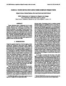
Finally, we highlight some specific examples of previous work that have been influential in the design of the proposed tempo induction method. Our work is similar in spirit to the computationally efficient multipitch estimation model proposed in [?]. In that paper, the authors showed how previous, more complicated, algorithms for multiple pitch detection could be simplified, improving both speed of computation and complexity without affecting accuracy. The idea of a cumulative beat histogram based on self similarity was originally proposed for characterizing rhythm for genre classification [?] as well as beat strength [?]. Another influential idea was the use of cross-correlation of “ideal” pulse sequences corresponding to a particular tempo and downbeat location with the onset strength signal. This approach was used for efficient tempo and beat tracking in audio recordings [?]. One of the issues facing tempo induction is that algorithms frequently make octave errors, i.e. they estimate the tempo to be either half or twice (a third or thrice) the actual ground truth tempo [?, ?]. It is frequently the case that this ambiguity also exists with human tapping; selecting the right tempo between two integer-related candidates is challenging. Recently machine learning techniques for estimating tempo classes (“slow”, “medium”, “fast”) [?] have been proposed and used for reducing octave errors for example by using the estimated class to create a prior to constrain the tempo estimation [?]. Our goal was to take these concepts, simplify each step, and combine them in an easily-reproducible algorithm. 2. ALGORITHM The proposed approach (shown in Figure 1) follows a relatively common architecture with the explicit design goal to simplify each step as much as possible without losing accuracy. For example, unlike many existing tempo estimation and beat tracking algorithms we do not utilize multiple frequency bands, perform peak picking during the onset strength signal calculation, employ dynamic programming, utilize complex probabilistic modeling based on musical structure, and our use of machine learning is simple and limited. The following sections describe each step. We provide two open-source implementations of the proposed algorithm. The first is in C++ and is part of the Marsyas audio processing framework [?]. The second is in Python and is a less efficient stand-alone reference implementation. We created two implementations to test the reproducibility of the description of the algorithm, as this is an increasingly important facet of research [?]. Both versions are available in the Marsyas SVN1 source repository, with the final version being revision 4953. All evaluation scripts and ground truth data are also included in the svn repository. Interested readers can contact the authors for details. 2.1. Onset Strength Signal The first step is to compute a time-domain onset strength signal (OSS) from the audio input signal. The OSS is at a lower sampling rate and should have high values at the locations where there are rhythmically salient events that are termed “onsets”. Beats tend to be located near onsets and can be viewed as a semi-regular subset of the onsets. A large number of onset detection functions have been proposed in the literature [?, ?]. In most cases, they measure some form of change in either energy or spectral content. In some cases, multiple onset detection functions are computed and are either treated separately for periodicity detection or combined to a single 1

http://sourceforge.net/p/marsyas/code/

Onset Strength Signal

Input, Overlap

Log Power Spectrum

Flux

Beat Histogram

Overlap

Autocorr.

Cumulative BH

Filter

Enhance harm. tempos EBH

8 cand. tempos Beat Phase

Evaluate pulse trains

Select best cands

Cumulative P BH

TP1 HB TP2 HB

TEBH

Doubling Heuristic

final tempo

Fig. 1: Dataflow diagram of the tempo induction algorithm

OSS. After experimentation with several choices we settled on a simple onset detection function that worked better than the alternatives and can be applied directly to the log-magnitude spectrum. More specifically, we sum the log-magnitudes of the frequency bins [?, ?] that have a positive change in log-magnitude over time:

OSSpre (n) =

N −1 X

(LP (f, n) − LP (f, n − 1)) · IP F (f, n)

f =0

LP (f, n) = ln (1 + 1000.0 · |X(f, n)|) ( 0 if |X(f, n)| − |X(f, n − 1)| ≤ 0 IP F (f, n) = 1 otherwise

(1)

where |X(f )| is the magnitude spectrum of the Fourier transform at frame n and frequency bin f , and IP F (f, n) is an indicator function selecting the frequency bins in which there is a positive change in log-magnitude. A Hamming window is applied before computing the Fourier transform. For the computation of the log-magnitude spectrum a window size of 256 samples at 44100 Hz sampling rate with a hop size of 128 samples is used. OSSpre is further low-pass filtered with a 7th -order FIR filter with a cutoff of 30 Hz, using the Hamming window design method to create the final OSS. 2.2. Periodicity Detection The filtering and the subsequent periodicity estimation is performed on sequences of 2048 samples of the OSS corresponding to segments of approximately 6 seconds of the original audio, also used in [?]. The hop size of the onset strength signal is 128 OSS samples corresponding to approximately 0.37 seconds. Each analysis frame of the OSS is denoted by m, with a total of M frames. Autocorrelation is applied to the onset strength signal to determine the different time lags in which the OSS is self similar. The lag (x-axis) of the peaks in the autocorrelation function will correspond to the dominant periodicities of the signal which in many cases will be harmonically related (integer multiples or ratios) to the actual underlying tempo. We utilize the “generalized autocorrelation” function [?] whose computation consists of zeropadding to double the length, computing the discrete Fourier transform of the signal, magnitude compression of the spectrum, followed by an inverse discrete Fourier transform: Am (t) = DF T −1 (|DF T (OSS(m))|k )

(2)

The parameter k controls the frequency domain compression. Normal autocorrelation has a value of k equal to 2 but it can be advantageous to use a smaller value [?]. The peaks of the autocorrelation

function tend to get narrower with smaller values of k resulting in better lag resolution. At the same time for low values of k the performance deteriorates as there is more noise sensitivity. We have empirically found k = 0.5 to be a good compromise between lagdomain resolution and sensitivity to noise.The generalized autocorrelation of the signal is subsequently warped and accumulated into a beat histogram (or periodicity vector). Unlike some of the previous autocorrelation-based approaches [?] in which peak picking is applied in the autocorrelation domain, we map all the values of the autocorrelation function to the Beat Histogram. More specifically each value of the generalized autocorrelation function is mapped to a corresponding BPM (beats-per-minute) value based on the lag t. b=

60.0 t

· Sr

(3)

where t is the time lag (in samples), Sr is the signal rate of the OSS, and b is subsequently quantized to an integer value ˆb in fractions of a beat (we use 0.25 BPM). It is possible that multiple lags t map to the same quantized ˆb value. The periodicity vector for the current OSS frame m is therefore created by averaging all the generalized autocorrelation values that map to quantized periodicity ˆb expressed in quarter BPM. Hm (ˆb) =

1 |Sˆ | b

P

l∈Sˆ b

Am (t)

(4)

where Am (t) is the generalized autocorrelation value of the onset strength signal at lag t in frame m, and Sˆb is the set of time lags t that map to quantized periodicity ˆb. Some of the values of the periodicity vector do not have any lag mapped to them. Their values are linearly interpolated from their neighbors. The beat histogram BH accumulates these periodicity vectors (between 50 and 200 BPM) over time: BHm (ˆb) =

M X

Hm (ˆb)

(5)

m=1

The BH will contain peaks at integer multiples of the underlying tempo as well as other dominant periodicities related to rhythmic subdivisions. To boost harmonically related peaks a time stretched version of the BH by a factor of 0.5 is added to the original resulting in an enhanced BH (EBH): EBHm (ˆb) = BHm (ˆb) + BHm (0.5 · ˆb)

(6)

The peaks of the cumulative EBH typically correspond to the main rhythmic periodicities present in the signal. The BPM values corresponding to the top 8 peaks (a value is considered a peak if it is larger than the values of a neighborhood of ±1.5 BPM around it) in the EBH of OSS frame m between 50 and 180 BPM are used as the tempo candidates examined in the following step of periodicity detection using pulse regularity. 2.3. Periodicity Detection using pulse regularity Once the candidate tempos from the EBH have been identified for a 6-second frame of the OSS, they are evaluated by correlating the OSS signal with an ideal expected pulse train that is shifted in time by different amounts. As shown by Laroche [?] this corresponds to a least-square approach of scoring candidate tempos and downbeat locations assuming a constant tempo during the analyzed 6 seconds. The cross-correlation with an impulse train can be efficiently performed by only multiplying the non-zero values, significantly reducing the cost of computation.

Given a candidate tempo period in samples P and a candidate phase location φ (the time instance a beat occurs) associated with OSS frame m, we create a sequence of 4 pulses as follows: IP,φ = φ + kP

k = 0, . . . , 3

(7)

In addition a series of secondary pulses with weight 0.5 are added to the ideal impulse train spaced by both 2P and 1.5P . These capture the common integer relations based on meter. When scoring a particular tempo candidate the resulting impulse signal is crosscorrelated with the OSS for all possible phases φ. If we denote ρc (φ, m) as the vector of cross-correlation values for all phases φ and candidate tempo c in window m, we can then score each tempo candidate with highest cross correlation value over all possible φ: SCv (c, m) = var(ρc (φ, m)) φ

SCx (c, m) = max(ρc (φ, m))

(8)

φ

These two score vectors are normalized so that they sum to 1 and added to yield the final scores for each tempo candidate. SCx (c, m) SCv (c, m) SC(c, m) = P +P c SCx (c, m) c SCv (c, m)

(9)

The SC(c, m) vector is also normalized such that its sum is 1. The highest score tempo candidate is selected for frame m and accumulated in a pulse regularity beat histogram P BH, which is initialized as 0. We define the argmax of SC(c, m) as ca (m). P BH(ca (m), m) = P BH(ca (m), m − 1) + SC(c, m)

(10)

2.4. Doubling heuristic Finally we consider three possible candidate tempos based on the cumulative EBH and P BH at the end of the audio file. The first candidate is the tempo corresponding to the highest peak of the enhanced self-similarity beat histogram, TEBH . The other two candidates correspond to the two highest peaks of the pulse regularity beat histogram, TP1 BH and TP2 HB . It was empirically observed that the tempo corresponding to the highest peak of the PBH tends to be the best estimate. However there are cases when one of the other candidates is a better choice and also frequently a pair of candidates has an integer ratio of 2 (with a tolerance parameter of ±4% BPM). The presence of such a pair is a strong indicator that one of them is the correct tempo but the question remains which one to pick. We use a simple tempo threshold to decide which of the doubling pair is the final predicted tempo. If we denote the lowest candidate of the doubling pair TL (it can be any of the three tempo candidates), and TH the higher tempo candidate the heuristic is:   arg maxT P BH no doubling pair Tf inal = 2 ∗ TL (11) TL 68 L L The doubling threshold of 68 BPM was determined using very simple machine learning (a decision tree) and an oracle approach based on the ground truth data. The “feature” was the lowest tempo candidate of the pair and the desired outcome was whether to double or not. This can be viewed as an extremely simplified version of the more complex machine learning approaches that have been proposed in the literature [?, ?, ?].

ACM MIRUM ISMIR04 SONG BALLROOM HAINSWORTH GTZAN GENRES Dataset average Total average

files 1410 465 698 222 1000 759 3795

marsyas 65.2 58.5 61.3 66.7 73.6 65.1 66.0

gkiokas 66.0 56.8 60.0 64.4 70.3 63.5 64.8

ACM MIRUM ISMIR04 SONG BALLROOM HAINSWORTH GTZAN GENRES Dataset average Total average

files 1410 465 698 222 1000 759 3795

marsyas 87.9 83.4 89.3 82.0 90.1 86.5 87.8

gkiokas 89.6 90.8 94.4 84.7 92.0 90.3 91.0+

zplane 64.5 56.1 64.2 69.8 67.664.5 64.6

klapuri 62.6 57.8 62.3 71.6 68.7 64.6 64.1

echonest 67.6 57.0 55.2 66.7 66.762.6 63.7

ibt 57.946.762.0 72.5 59.859.8 58.6-

qm vamp 58.842.864.0 72.5 57.159.1 58.2-

scheirer 49.542.652.649.155.649.9 50.8-

echonest 85.2 78.5 84.1 85.6 85.7 83.8 84.3-

ibt 86.0 76.6 87.8 82.0 86.1 83.7 85.0

qm vamp 85.3 77.6 86.0 83.8 84.9 83.5 84.3-

scheirer 71.464.373.665.375.670.1 71.7-

(a) Accuracy 1 results zplane 86.5 82.4 92.1 82.4 87.7 86.2 87.1

klapuri 88.5 89.2 90.1 84.2 90.9 88.6 89.3

(b) Accuracy 2 results. Table 1: Tempo accuracy, results given in %. The + and - indicate that the difference between this algorithm and Marsyas is statistically significant. Bold numbers indicate the best-performing algorithm for this dataset. The “Dataset average” row is the mean of the algorithm’s accuracy between all datasets, while the “Total average” is the accuracy over all datasets summed together.

3. EVALUATION The proposed algorithm (marsyas) was tested against 7 other tempo induction algorithms on 5 datasets of 44100 Hz, 16-bit audio files. As with other tempo evaluations, two accuracy measures are used: Accuracy 1 is the percent of estimates which are within 4% BPM of the ground-truth tempo, and Accuracy 2 is the percent of estimates which are within 4% of a multiple of 13 , 21 , 1, 2, or 3 times the ground-truth tempo. Following the measure of statistical significance used in [?, ?], we tested the accuracy of each algorithm against our accuracy with McNemar’s test using a significance value of p < 0.01. Table 1 lists some representative results comparing the proposed method with both commercial and academic tempo estimation methods. For algorithms that had variants such as ibt, we selected the best performing variant. As can be seen marsyas has the best Accuracy 1 although the difference with the other top performing algorithms is not statistically significant. We briefly describe the algorithms and datasets. gkiokas [?] has the best Accuracy 2 performance. It is significantly more complicated than our proposed approach as it uses a constant-Q transform, harmonic/percussive separation algorithm, modeling of metrical relations, and dynamic programming. zplane is a commercial beat-tracking algorithm 2 used in a variety of products such as Ableton Live and was designed for whole songs rather than snippets. klapuri [?] uses a bank of comb filters and simultaneously estimates three facets of the audio: the atomic tatum pulses, the tactus tempo, and the musical measures using a probabilistic formulation. It is also more complicated than our proposed method. echonest is the development build of version 3.2 of the Echo Nest track analyzer3 . The algorithm is based on a trained model and is optimized for speed and generalization. ibt [?, ?] uses multiple agents which create hypotheses about tempo and beats that are continuously evaluated using a continuous onset detection function. qm-vamp [?] is implemented as part of the Vamp audio plugins4 which outputs a series of varying tempos. To compare this set to the single fixed 2 [aufTAKT]

V3, http://www.beat-tracking.com http://developer.echonest.com/ 4 http://vamp-plugins.org/ 3

ground-truth tempo, we calculated the weighted mean of those varying tempos, where each BPM is weighted by the length for which that tempo is held. scheirer [?] was created in 1996 and uses a bank of parallel comb filters for tempo estimation. It was selected as a baseline to observe how tempo induction has improved over time. ACM MIRUM was originally gathered with crowd-sourced annotations [?], but was further processed by [?] to remove songs for which the tempo annotations differed significantly. ISMIR04 SONG and BALLROOM arose from the 2004 competition conducted in [?]. HAINSWORTH came from [?]. Tempo annotations were recently added to the GENRES dataset [?] (10 genres, 100 tracks per genre) and is available in the Marsyas SVN repository in the file collections/genres tempos.mf 4. CONCLUSIONS We have presented a simple, effective algorithm for tempo estimation from audio signals. It exploits self-similarity and pulse regularity using ideas from previous work that have been reduced to their bare essentials. Each step is relatively simple and there are only a few parameters to adjust. A thorough experimental evaluation with the largest number of data sets and music track to date, shows that our proposed method has excellent performance that is statistically indistinguishable from the top performing algorithms including two commercial systems. We hope that providing a detailed description of the steps, open source implementations, and the scripts used for the evaluation experiments will assist reproducibility and stimulate more research in rhythmic analysis. In the future we plan to use the proposed tempo estimation method as part of beat tracking and rhythmic pattern detection algorithms.

Acknowledgements Part of this work was performed when the first author was at Google Research in 2011 and informed by discussion with D. Lyon and D. Ross. We also would like to thank T. Jehan, from Echonest, A. Lerch, from z-plane, A. Klapuri, A. Gkiokas, and G. Peeters for providing their algorithms and helping us set them up for evaluation.

5. REFERENCES [1] P. Grosche, M. M¨uller, and C. S. Sapp, “What makes beat tracking difficult? a case study on chopin mazurkas,” in ISMIR, 2010, pp. 649–654. [2] A.M. Wing and A.B. Kristofferson, “Response delays and the timing of discrete motor responses,” Attention, Perception, & Psychophysics, vol. 14, no. 1, pp. 5–12, 1973. [3] B.H. Repp, “Sensorimotor synchronization: A review of the tapping literature,” Psychonomic Bulletin & Review, vol. 12, no. 6, pp. 969–992, 2005. [4] M. Goto and Y. Muraoka, “A beat tracking system for acoustic signals of music,” in ACM Multimedia, 1994, pp. 365–372. [5] E. D. Scheirer, “Tempo and beat analysis of acoustic musical signals,” The Journal of the Acoustical Society of America, vol. 103, no. 1, pp. 588–601, 1998. [6] F. Gouyon, A. Klapuri, S. Dixon, M. Alonso, G. Tzanetakis, C. Uhle, and P. Cano, “An experimental comparison of audio tempo induction algorithms,” Audio, Speech, and Language Processing, IEEE Transactions on, vol. 14, no. 5, pp. 1832 – 1844, September 2006. [7] J. Zapata and E. G´omez, “Comparative evaluation and combination of audio tempo estimation approaches,” in AES conference on Semantic Audio, July 2011. [8] S. Hainsworth, “Beat tracking and musical metre analysis,” Signal processing methods for music transcription, pp. 101– 129, 2006. [9] T. Tolonen and M. Karjalainen, “A computationally efficient multipitch analysis model,” Speech and Audio Processing, IEEE Transactions on, vol. 8, no. 6, pp. 708–716, 2000. [10] G. Tzanetakis and P. Cook, “Musical genre classification of audio signals,” Speech and Audio Processing, IEEE transactions on, vol. 10, no. 5, pp. 293–302, 2002. [11] G. Tzanetakis, G. Essl, and P. Cook, “Human perception and computer extraction of musical beat strength,” in Proc. DAFx, 2002, vol. 2. [12] J. Laroche, “Efficient tempo and beat tracking in audio recordings,” J. Audio Eng. Soc, vol. 51, no. 4, pp. 226–233, 2003. [13] P. Grosche, M. Muller, and F. Kurth, “Cyclic tempogram – a mid-level tempo representation for music signals,” in ICASSP, March, pp. 5522–5525. [14] G. Peeters, “Time variable tempo detection and beat marking,” in Proc. of the International Computer Music Conference (ICMC), Barcelona, September 2005. [15] J. Hockman and I. Fujinaga, “Fast vs slow: Learning tempo octaves from user data.,” in ISMIR, 2010, pp. 231–236. [16] A. Gkiokas, V. Katsouros, and G. Carayannis, “Reducing tempo octave errors by periodicity vector coding and svm learning,” in ISMIR, 2012, pp. 301–306.

[17] G. Tzanetakis, “Marsyas-0.2: a case study in implementing music information retrieval systems,” Intelligent Music Information Systems. IGI Global, 2007, http://marsyas.info. [18] P. Vandewalle, J. Kovacevic, and M. Vetterli, “Reproducible research in signal processing,” Signal Processing Magazine, IEEE, vol. 26, no. 3, pp. 37–47, May 2009. [19] J.P. Bello, L. Daudet, S. Abdallah, C. Duxbury, M. Davies, and M.B. Sandler, “A tutorial on onset detection in music signals,” Speech and Audio Processing, IEEE Transactions on, vol. 13, no. 5, pp. 1035–1047, 2005. [20] S. Dixon, “Onset detection revisited,” in DAFx, 2006, vol. 120, pp. 133–137. [21] P. Grosche and M. Muller, “Extracting predominant local pulse information from music recordings,” Audio, Speech, and Language Processing, IEEE Transactions on, vol. 19, no. 6, pp. 1688–1701, Aug. [22] G. Peeters and J. Flocon-Cholet, “Perceptual Tempo Estimation using GMM-Regression,” in MIRIUM, Nara, Japan, 2012. [23] L. Gillick and S. Cox, “Some statistical issues in the comparison of speech recognition algorithms,” in ICASSP, 1989, pp. 532–535. [24] A. Gkiokas, V. Katsouros, G. Carayannis, and T. Stajylakis, “Music tempo estimation and beat tracking by applying source separation and metrical relations,” in ICASSP. IEEE, 2012, pp. 421–424. [25] A.P. Klapuri, A.J. Eronen, and J.T. Astola, “Analysis of the meter of acoustic musical signals,” Audio, Speech, and Language Processing, IEEE Transactions on, vol. 14, no. 1, pp. 342 – 355, January 2006. [26] J. L. Oliveira, F. Gouyon, L. G. Martins, and L. P. Reis, “Ibt: A real-time tempo and beat tracking system.,” in ISMIR. 2010, pp. 291–296, International Society for Music Information Retrieval. [27] J.L. Oliveira, M.E.P. Davies, F. Gouyon, and L.P. Reis, “Beat tracking for multiple applications: A multi-agent system architecture with state recovery,” Audio, Speech, and Language Processing, IEEE Transactions on, vol. 20, no. 10, pp. 2696 –2706, December 2012. [28] M. E. P. Davies and M. D. Plumbley, “Context-dependent beat tracking of musical audio.,” IEEE Transactions on Audio, Speech & Language Processing, vol. 15, no. 3, pp. 1009–1020, 2007. [29] M. Levy, “Improving perceptual tempo estimation with crowdsourced annotations.,” in ISMIR, 2011, pp. 317–322. [30] S. W. Hainsworth, Techniques for the Automated Analysis of Musical Audio, Ph.D. thesis, University of Cambridge, UK, September 2004.