IEEE/ACM TRANSACTIONS ON AUDIO, SPEECH, AND LANGUAGE PROCESSING, VOL. 22, NO. 12, DECEMBER 2014
1765
Streamlined Tempo Estimation Based on Autocorrelation and Cross-correlation With Pulses Graham Percival, Member, IEEE, and George Tzanetakis, Senior Member, IEEE
Abstract—Algorithms for musical tempo estimation have become increasingly complicated in recent years. These algorithms typically utilize two fundamental properties of musical rhythm: some features of the audio signal are self-similar at periods related to the underlying rhythmic structure, and rhythmic events tend to be spaced regularly in time. We present a streamlined tempo ) that distills ideas from previous work estimation method ( by reducing the number of steps, parameters, and modeling assumptions while retaining good accuracy. This method is designed for music with a constant or near-constant tempo. The proposed method either outperforms or has similar performance to many existing state-of-the-art algorithms. Self-similarity is captured through autocorrelation of the onset strength signal (OSS), and time regularity is captured through cross-correlation of the OSS with regularly spaced pulses. Our findings are supported by the most comprehensive evaluation of tempo estimation algorithms to date in terms of the number of datasets and tracks considered. During the process we have also corrected ground truth annotations for the datasets considered. All the data, the annotations, the evaluation code, and three different implementations (C++, Python, MATLAB) of the proposed algorithm are provided in order to support reproducibility. Index Terms—Audio signal processing, music information retrieval, rhythm analysis, tempo induction.
I. INTRODUCTION
T
EMPO estimation is a fundamental problem in music information retrieval (MIR), vital for applications such as music similarity and recommendation, semi-automatic audio editing, automatic accompaniment, polyphonic transcription, beat-synchronous audio effects, and computer assisted DJ systems. Typically, automatic analysis of rhythm consists of two main tasks: tempo estimation and beat tracking. The goal of tempo estimation is to automatically determine the rate of musical beats in time. Beats can be defined as the locations in time where a human would “tap” their foot while listening to a piece of music. Beat tracking is the task of determining the locations of these beats in time, and is considerably harder in music in which the tempo varies over time [1]. Both of these topics have received considerable attention and there is a large body of published literature exploring various approaches to solving them automatically. Manuscript received July 28, 2013; revised March 04, 2014; accepted August 10, 2014. Date of publication August 18, 2014; date of current version August 26, 2014. The associate editor coordinating the review of this manuscript and approving it for publication was Prof. Bozena Kostek. G. Percival is with the National Institute of Advanced Industrial Science and Technology, Tsukuba 305-8568, Japan (e-mail:
[email protected]). G. Tzanetakis is with the Department of Computer Science, University of Victoria, Victoria, BC V8W3P6, Canada (e-mail:
[email protected]). Digital Object Identifier 10.1109/TASLP.2014.2348916
In this work, we focus solely on the task of tempo estimation or tempo induction (another term frequently used for the same task). Algorithms for tempo estimation have become, over time, increasingly more complicated. They frequently contain multiple stages, each with many parameters that need to be adjusted. This complexity makes them less efficient, harder to optimize due to the large number of parameters, and difficult to replicate. Our goal has been to streamline the tempo estimation process by reducing the number of steps and parameters without affecting the accuracy of the algorithm. An additional motivation is that tempo estimation is a task that most human listeners (even without musical training) can do reasonably well. Therefore, it should be possible to model this task without requiring complex models of formal musical knowledge, although mimicking the basic human perception remains a challenging task. One challenge particular to tempo estimation is that, although most untrained listeners can track the overall speed of most music, their estimates can often differ by an integer multiple. For example, a march (a song with a very clear and steady beat, specifically designed to permit non-musically-trained soldiers to walk at the same speed) could be perceived as “one two three four, one two three four” or “one and two and, one and two and.” Another famous example is a waltz (a formal European dance, again specifically designed to permit easy perception of the beats), which could be perceived as “one two three, one two three” or “one and a, one and a.” If the words in all the above examples are said at the same rate (say, 150 words per minute) but the perception of a “beat” is restricted to the numbers, then the potential Beats Per Minute (BPM) of the march are 150 and 75, while the potential tempos of the waltz are 150 and 50. In many cases, it is not meaningful to say that either one of those pairs of numbers are incorrect. After an early period in which systems were evaluated individually on small private datasets, since 2004 there have been three public datasets that have been frequently used to compare different approaches. We have conducted a thorough experimental investigation of multiple tempo estimation algorithms which uses two additional datasets to the classic three datasets. We show that our proposed streamlined tempo estimation method ( ) demonstrates state-of-the-art performance that is statistically very close to the best performing systems we evaluated. The code of our algorithm, as well as the scripts used for the experimental comparison of all the different systems considered, is available as open source software in three different implementations (C++, Python, MATLAB). Moreover, all the datasets used and associated ground truth are publicly available. By supporting reproducible digital signal processing research we hope to stimulate further experimentation in tempo estimation and automatic rhythmic analysis in general.
2329-9290 © 2014 IEEE. Personal use is permitted, but republication/redistribution requires IEEE permission. See http://www.ieee.org/publications_standards/publications/rights/index.html for more information.
1766
IEEE/ACM TRANSACTIONS ON AUDIO, SPEECH, AND LANGUAGE PROCESSING, VOL. 22, NO. 12, DECEMBER 2014
A. Related work The origins of work in tempo estimation and beat tracking can be traced to research in music psychology. There are some indications that humans solve these two problems separately. In the early (1973) two-level timing model proposed by [2], separate mechanisms for estimating the period (tempo) and phase (beat locations) are proposed by examining data from tapping a Morse key. A recent overview article of the tapping literature [3] summarizes the evidence for a two-process model that consists of a slow process which measures the underlying tempo and a fast synchronization process which measures the phase. Work in automatic beat tracking started in the 1980s but mostly utilized symbolic input, frequently in the form of MIDI (Musical Instrument Digital Interface) signals. In the 1990s the first papers investigating beat tracking of audio signals appeared. A real-time beat tracking system based on a multiple agent architecture was proposed in 1994 [4]. Each agent corresponded to a particular tempo/phase hypothesis and was scored based on how it was supported by the analyzed audio data consisting of a discrete set of automatically detected pulses corresponding to onsets. Another influential early paper described a method that utilized comb filters to extract beats from polyphonic music [5]. It also introduced the idea of continuous processing of the audio signals rather than discrete onset locations. There has been an increasing amount of interest in tempo estimation for audio signals in recent years. A large experimental comparison of various tempo estimation algorithms was conducted in 2004 as part of the International Conference on Music Information Retrieval (ISMIR) and presented in a journal article [6]. A more recent experimental comparison of 23 algorithms was performed in 2011, giving a more in-depth statistical comparison between the methods considered [7]. The original 2004 study established the evaluation methodology and data sets that have been used in the majority of subsequent work, including ours. There has been a growing concern that algorithms might be over-fitting these data sets created in 2004. In our work we have expanded both the number of datasets and music tracks in order to make the evaluation results more reliable. Although there is considerable variety in the details of different algorithms, there are some common stages such as onset detection and period analysis that are shared by most of them. An overview of different algorithms and the type of rhythmic models and processing steps they employ can be found in [8]. A fundamental concept in tempo estimation algorithm is the notion of onsets. Onsets are the locations in time where significant rhythmic events such as pitched notes or transient percussion events take place. Some of the previous algorithms use hard onset decisions, i.e. their input is a discrete list of onset locations over time [4], [9], [10], [11]. An alternative is to use a more continuous representation in which a “soft” onset strength value is provided at a regular time locations. The resulting signal is frequently called the onset strength signal (OSS) [12], [13], [14]. The next step is to determine the dominant periods based on the extracted onset information. The previous approaches for period detection fall into some common groups. Histogramming methods are based on computing inter-onset intervals (IOI) from discrete lists of onset
locations, that are then accumulated in a histogram whose bins correspond to the periods of interest [11]. In autocorrelation methods [15], [16], [17] the onset strength is analyzed periodically typically at intervals of several seconds by computing the autocorrelation function of each interval. The peaks of the autocorrelation function should correspond to the period length of the different metrical levels of the underlying rhythm. Oscillating filter approaches use the input data to either adapt a non-linear oscillator whose frequency represents the tempo and whose phase represents the beat locations [18] or a bank of resonating filters at fixed periods [5], [19]. In all these cases, the typical output is a representation called a beat histogram or beat spectrum which captures the amount of confidence or beat strength [16] for each candidate tempo for the data that has been analyzed. A generalization of this representation is used in multiple agent approaches [4], [20], [14], [21]. Multiple tempo and pulse hypotheses are considered in parallel and tracked over time. In some cases multiple onset detection function or even different beat trackers can be utilized simultaneously. Each “agent” keeps track of its score and at the end the “agent” with the highest score is selected as the estimated tempo. In order to track changes in tempo and beat locations over time, a common approach is to utilize dynamic programming [22]. Finally, other approaches [12], [23], [19] assume that there is a probabilistic model that characterizes the generation of rhythmic events. The goal of such algorithms is to estimate the parameters of this generative process, typically using standard estimation procedures such as Kalman filtering, Markov Chain Monte Carlo, or sequential Monte Carlo (particle filtering) algorithms [24]. Finally, we highlight examples of previous work that have been influential in the design of . Our work is similar in spirit to the computationally efficient multipitch estimation model proposed in [25]. In that work, the authors showed how previous, more complicated, algorithms for multiple pitch detection could be simplified, improving both speed of computation and complexity without affecting accuracy. An influential idea has been the use of cross-correlation of “ideal” pulse sequences corresponding to a particular tempo and downbeat locations with the onset strength signal [26]. The use of variance to “score” the different period candidates when cross-correlating with pulse sequences with different phases was inspired by the phase autocorrelation matrix approach proposed by [27]. One of the issues facing tempo estimation is that algorithms frequently make octave errors, i.e. they estimate the tempo to be either half or twice (or a third or thrice) the actual ground truth tempo [28], [29]. This ambiguity is also common with human tapping. Our work only deals with halved or doubled tempos. Recently, machine learning techniques for estimating tempo classes (“slow”, “medium”, “fast”) [30], [31] have been proposed and used for reducing octave errors, for example by using the estimated class to create a prior to constrain the tempo estimation process [32]. Our goal has been to take these concepts, simplify each step, and combine them in an easily-reproducible algorithm. B. Improvements over previous paper An earlier version of the algorithm described in this article was presented at the International Conference on Audio, Speech
PERCIVAL AND TZANETAKIS: STREAMLINED TEMPO ESTIMATION BASED ON AUTOCORRELATION
1767
Fig. 2. Dataflow diagram for OSS calculation. Left: processing blocks. Right: example of data.
Fig. 1. Dataflow diagram of the tempo estimation algorithm. Left: processing blocks. Right: type of data, and an example of the data.
and Signal Processing (ICASSP) in 2013 [33]. In this work we have further simplified the processing steps of the method. More specifically, we no longer utilize Beat Histograms and do not retain a separate tempo candidate from the Beat Histogram. Instead, all cumulative processing as well as the detection of the tempo candidate are done directly in the generalized autocorrelation lag domain. In addition, the description of the algorithm has been expanded with more figures, text, and equations improving understanding. We also provide updated experimental results based on corrected ground truth and implement a more sophisticated machine learning scheme to determine whether the tempo should be doubled. Finally, we provide three different open source implementations (C++, Python and MATLAB) that have all been tested and provide identical results. Together with the datasets and associated ground truth, these implementations support reproducibility which is increasingly becoming important in signal processing research [34]. II. ALGORITHM The proposed approach follows a relatively common architecture with the explicit design goal to simplify each step as much as possible without losing accuracy. There are three main stages to the algorithm, as shown in Fig. 1. The initial audio input has a sampling rate of Hz. 1) Generate Onset Strength Signal (OSS) The time-domain audio signal is converted into a signal which (ideally) indicates where humans would perceive onsets to occur. The OSS is also at a lower sampling rate; Hz. 2) Beat Period Detection The OSS signal is split into overlapping windows roughly 5.9 seconds long, and each segment is analyzed for the tempo. After examining the range of annotated tempos in the datasets, we chose a minimum tempo of 50 BPM and maximum tempo of 210 BPM. The output of this step is a single tempo estimate, expressed as a lag of samples (of
). The sampling rate of these tempo estimates is Hz. 3) Accumulator and overall estimate The tempo estimates are accumulated, and at the end of the track an overall estimate (in BPM) is derived from the accumulated results. A heuristic is used to determine whether this estimate is correct or whether it should be halved or doubled. In contrast to many existing tempo estimation and beat tracking algorithms, we do not utilize multiple frequency bands [19], perform peak picking during the onset strength signal calculation [9], employ dynamic programming [22], utilize complex probabilistic modeling based on musical structure [19], [23], and our use of machine learning is simple and limited. The following sections describe each of the main processing steps in detail. A. Generate Onset Strength Signal (OSS) The first step is to compute a time-domain Onset Strength Signal (OSS) from the audio input signal. The final OSS is at a lower sampling rate than the audio input, and should have high values at the locations where there are rhythmically salient events that are termed “onsets.” Beats tend to be located near onsets and can be viewed as a semi-regular subset of the onsets. A large number of onset detection functions have been proposed in the literature [35], [10]. In most cases, they measure some form of change in either energy or spectral content. In some cases, multiple onset detection functions are computed and are either treated separately for period detection or combined to a single OSS [5], [17]. After experimentation with several choices we settled on a simple onset detection function that worked better than the alternatives and can be applied directly to the log-magnitude spectrum. The dataflow diagram and an example are shown in Fig. 2. 1) Overlap: We begin by segmenting the audio (originally at 44100 Hz sampling rate) into overlapping frames of 1024 samples with a hop size of 128 samples. This produces a set of frames with a sampling rate of Hz. 2) Log Power Spectrum: Each frame is multiplied by a Hamming window function, then we compute the magnitude spectrum with the Discrete Fourier Transform. We define
1768
IEEE/ACM TRANSACTIONS ON AUDIO, SPEECH, AND LANGUAGE PROCESSING, VOL. 22, NO. 12, DECEMBER 2014
as the magnitude spectrum at frame and frequency bin . We further define as the log-power magnitude spectrum, (1) 3) Flux: We calculate the spectral flux by summing the logmagnitudes of the frequency bins [8], [17] that have a positive change in log-magnitude over time. is the number of FFT bins representing positive frequencies, . The DC-offset FFT bin 0 is omitted from the spectral flux calculation. is an indicator function selecting the frequency bins in which there is a positive change in log-magnitude,
(2) This flux calculation reduces the dataflow from a series of frames (of 257 samples) at 344.5 Hz to a 1-dimensional signal at 344.5 Hz. 4) Low-pass filter: The signal is further low-pass filtered with a 14th-order FIR filter with a cutoff of 7 Hz, designed with the Hamming window method. 7 Hz was used as it is twice the maximum BPM value of 210 BPM (or 3.5 Hz). The output of this filter is our Onset Strength Signal. Subsequent stages of our algorithm (Section II-B and Section II-C) use this to estimate the tempo of the audio, but the OSS could also serve as the initial step to an onset detection or beat tracking algorithm. B. Beat Period Detection Having generated the OSS, we now estimate the tempo for each portion of audio. In particular, we examine frames of the OSS which are 2048 samples long. This corresponds to approximately 6 seconds of audio ( s), similarly to [17]. The hop size of the Onset Strength Signal is 128 OSS samples corresponding to approximately 0.37 seconds. Each analysis frame of the OSS is denoted by , with a total of frames. Therefore, the algorithm requires 5.9 seconds for an initial estimate of the tempo and updates this tempo estimate approximately once every 0.37 seconds. The dataflow diagram is shown in Fig. 3. 1) Overlap: We begin by segmenting the OSS (originally at 344.5 Hz sampling rate) into overlapping frames of 2048 samples with a hop size of 128 samples. This produces a set of frames with a sampling rate of Hz. 2) Generalized Autocorrelation: Autocorrelation is applied to the OSS to determine the different time lags in which the OSS is self similar. The lag (x-axis) of the peaks in the autocorrelation function will correspond to the dominant periods of the signal which in many cases will be harmonically related (integer multiples or ratios) to the actual underlying tempo. We utilize the “generalized autocorrelation” function [25] whose computation consists of zero-padding to double the length, computing the discrete Fourier transform of the signal, magnitude compression of the spectrum, followed by an inverse discrete Fourier transform: (3)
Fig. 3. Dataflow diagram for beat periods detection. The autocorrelation plots (2nd and 3rd down) only show the range of interest (98 to 414 samples).
The parameter controls the frequency domain compression and is the lag in OSS samples. Normal autocorrelation has a value of equal to 2 but it can be advantageous to use a smaller value [25]. The peaks of the autocorrelation function tend to get narrower with smaller values of , resulting in better lag resolution. At the same time, for low values of the performance deteriorates as there is more noise sensitivity. We have empirically found to be a good compromise between lag-domain resolution and sensitivity to noise. Our algorithm uses autocorrelation lag values for the remainder of the processing, but some readers may feel more comfortable dealing with BPM as that is how musicians discuss tempo. The BPM can be calculated from the autocorrelation lag: (4) 3) Enhance Harmonics: The autocorrelation has peaks corresponding to integer multiples of the underlying tempo as well as other dominant periods related to rhythmic subdivisions. To boost harmonically related peaks, two time-stretched version of the (by factors of 2 and 4) are added to the original re: sulting in an enhanced autocorrelation (5) 4) Pick peaks: The top 10 peaks in the enhanced autocorreare extracted; these are the tempo candidates for lation the scoring. Only peaks between the minimum and maximum autocorrelation lag are considered, (6) (7) 5) Evaluate pulse trains: Once the candidate tempos from the have been identified for a 2048-sample frame of the OSS, the candidates are evaluated by correlating the OSS signal with
PERCIVAL AND TZANETAKIS: STREAMLINED TEMPO ESTIMATION BASED ON AUTOCORRELATION
1769
index can extend as far (for example, at 60 BPM the as 8 seconds), that pulse is omitted from the cross-correlation. This adds a slight penalty to the maximum value of this crosscorrelation for tempos less than 71 BPM. When scoring a particular tempo candidate , the resulting impulse signal is cross-correlated with the OSS for all possible phases . We define , (9) as the vector of cross-correlation values for all phases and candidate tempo in OSS frame . The tempo candidates are then scored based on this vector. Two scoring functions are calculated: , the highest cross-correlation value over all possible , and , the variance of cross-correlation values over all possible , as suggested by [27]:
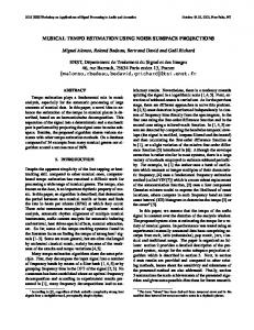
Fig. 4. Pulse trains used for evaluating the tempo candidates.
(10)
Fig. 5. Example of evaluating pulse trains. Top: one particular OSS frame. . Middle: pulse train for a tempo lag of 178 samples (116 BPM) with . Note Bottom: cross-correlation between the OSS and all that the hop-size of the beat period detection is 128 samples, so even though this particular frame will not involve the last portion of the OSS frame, that data will be used in a later frame.
an ideal expected pulse train that is shifted in time by different amounts. There are two inputs to the process: a frame of the OSS signal (before the generalized autocorrelation is calculated), and the 10 tempo candidates extracted from the . As shown by [26], this corresponds to a least-square approach of scoring candidate tempos and downbeat locations assuming a constant tempo during the analyzed 6 seconds. Our tempo algorithm is not concerned with downbeats, but we adopted it since this approach provided a useful way to evaluate candidate tempos. The cross-correlation with an impulse train can be efficiently performed by only multiplying the non-zero values, significantly reducing the cost of computation. Given a candidate tempo lag in OSS samples and a candidate phase location (the time instance a beat occurs), we create three sequences of pulses with : (8) Each sequence should be understood as a beat pattern corresponding to multiples of the candidate ; musically speaking, these capture common integer relationships based on meter. These three sequences are summed to form a single sequence, where has weight 1.0, and and have weight 0.5. The combined sequence is called . This process is shown in shown in Fig. 4. The impulse train is cross-correlated with the OSS frame , with . This is shown in Fig. 5. If an index of the impulse train falls outside the OSS frame
The rationale behind using the variance as a scoring criterion is that if the onset signal is relatively flat and there are no pronounced rhythmic events, there will be small variance in the cross-correlation values between the different “phases.” However if there are pronounced rhythmic onsets the variance will be high. These two score vectors are normalized so that they sum to 1 and are added to yield the final score for each tempo candidate in frame : (11) The highest scoring tempo lag candidate the frame :
is selected for (12)
The algorithm accumulates these estimates and makes a single overall estimate of the entire track (Section II-C), but the OSS and period detection method could be used to provide causal tempo estimates which could trigger events from recorded audio. If tempo updates are required more often than every 0.37 seconds, the hopsize could be reduced accordingly. However, these tempo estimates are not sufficient for beat tracking, as they make no attempt to track tempo estimates (and the offset for the pulse trains) from one frame to the next; in addition, our algorithm is more accurate when these estimates are accumulated for an entire audio track. C. Accumulation and overall estimate The final step of the algorithm is to accumulate all tempo lag estimates from each frame of the OSS. The dataflow diagram is shown in Fig. 6. 1) Convert to Gaussian: In most music, the tempo fluctuates slightly throughout the music. Even when the tempo is steady, the OSS and beat period detection calculations can result in a slightly different estimate . To accommodate these fluctuations, instead of accumulating a single value for , we create with and : a Gaussian curve (13)
1770
IEEE/ACM TRANSACTIONS ON AUDIO, SPEECH, AND LANGUAGE PROCESSING, VOL. 22, NO. 12, DECEMBER 2014
TABLE I CONFUSION MATRIX OF STEM-SVM3 TRAINING
version of the more complex machine learning approaches that have been proposed in the literature [32], [36], [31]. A somewhat more advanced algorithm ( ) uses a support vector machine (SVM) with a linear kernel to decide whether to output , , or . We use 3 features extracted from the tempo estimate accumulator . The first feature is the sum of values below the overall tempo lag estimate ; the second is the sum of values close to . In both cases, we consider 10 samples to be the threshold for the “area of interest.” The third feature is simply the candidate lag itself.
Fig. 6. Dataflow diagram for accumulation and overall estimate.
Using a fixed for different lag estimates results in a graduated range of tempo estimates in the BPM domain. Given a single lag estimate , the Gaussian is slightly biased towards higher tempos. In addition, slower tempos have a narrower range. To illustrate, we will give the range of BPMs covered by a tempo candidate lag samples. A Gaussian curve for an estimate of 60 BPM will cover to ; an estimate of 120 BPM will cover to ; and an estimate of 180 to . BPM will cover 2) Accumulator (sum): The for each frame is accumulated in a Tempo Estimate Accumulator . is a vector long enough to hold all possible autocorrelation lags, and is initialize to be 0, (14) 3) Pick peak: At the end of the audio track, we pick the index with the highest value in our tempo estimate accumulator , and convert it to a BPM value to be our overall tempo lag estimate . 4) Octave decider: Converting the tempo lag estimate directly into a tempo in BPM produces many estimates which are half the ground-truth and some which are double the ground-truth. This algorithm (with no tempo doubling or halving) shall be called as it serves as a baseline algorithm. In particular, out of 4011 files, 2100 are correct, while 1310 are half the ground-truth BPM and 208 are double the ground-truth. If we could accurately predict whether the tempo estimate should be multiplied by 1, or 2, the accuracy would jump from 52% to 85%; if we could decide between 1, 2, or 0.5, the accuracy would jump to 90.2%. The simplest possible improvement would be to set a threshold so that any tempo below it would be doubled. This algorithm ( ) should not be understood as a suggestion for practical use; rather, we present this method as a way of investigating the idea of automatic doubling. The doubling threshold of 71.9 BPM was determined using simple machine learning (a decision tree) and an oracle approach based on the ground truth data for training. The “feature” is the tempo candidate and the classification decision is whether to double or not. This can be viewed as an extremely simplified
(15) To train , we selected files for which doubling or not would produce the correct annotation. To train , we also selected files for which halving would produce the correct annotation. Of the 4011 files in total, an oracle approach of comparing the candidate to the ground-truth data revealed that 2045 files should not be doubled, 1344 should be doubled, and 622 annotations were incorrect regardless of doubling. We omitted the 622 incorrect answers and used the remaining 3369 files for training. was trained , a simple decision rule; the with Weka’s1 10-fold cross-validation accuracy was 78.0%. was trained with SMO, the traditional method of training SVM machines; the 10-fold cross-validation accuracy was 76.3%, with the confusion matrix shown in Table I. III. EVALUATION The proposed algorithm ( ) was tested against 7 other tempo estimation algorithms on 6 datasets of 44100 Hz, 16-bit audio files, comprising 4011 audio tracks in total. As with other tempo evaluations [6], [7], two accuracy measures are used: Accuracy 1 is the percent of estimates which are within 4% BPM of the ground-truth tempo, and Accuracy 2 is the percent of estimates which are within 4% of a multiple of , , 1, 2, or 3 times the ground-truth tempo. Following the measure of statistical significance used in [37], [7], we tested the accuracy of each algorithm against our accuracy with McNemar’s test, using a significance value of . The null hypothesis of this test is that if a pair of algorithms produces one correct and one incorrect answer for a certain audio track, there is an equal probability of each algorithm giving the correct answer. Given the number of instances where algorithm A is correct while algorithm B is incorrect, and the number of instances where B is correct and A is incorrect, the test statistic is . This statistic is compared to the distribution with 1 degree of freedom. 1http://www.cs.waikato.ac.nz/ml/weka/
PERCIVAL AND TZANETAKIS: STREAMLINED TEMPO ESTIMATION BASED ON AUTOCORRELATION
Fig. 7. Example of incorrect ground truth in BALLROOM dataset. The file .wav was annotated as being 124 BPM, but it is actually 116 BPM.
A. Datasets and Ground Truth Shared datasets are vital for the comparison of algorithms between different researchers, and the tempo induction community has been accumulating tempo-annotated audio collections starting with the MIREX tempo induction competition in 2004 [6]. However, in addition to having shared datasets, it is important that these datasets contain correctly-annotated ground truth. Testing algorithms on flawed data can produce inaccurate estimates of the algorithms’ accuracy in the best case, and in the worst case it may lead researchers to tweak parameters sub-optimally to produce a higher accuracy on the flawed data. Links to all of the datasets are available at our webpage to facilitate reproducible research (Section V). We found that three of the five datasets used in tempo induction experiments contained 4%–10% incorrect annotations, with the correct ground truth varying up to 30% away from the annotated ground truth. One example is shown in Fig. 7. Tempo collections which contain corrected data from previously published papers are indicated with a star *. To investigate the data annotations, we examined a subset of “questionable” tempo annotations. We defined “questionable” as “files for which two of the top three algorithms did not satisfy Accuracy 2.” This is very similar to the selective sampling method used in [38], [39], wherein the difficulty of beat tracking audio tracks is calculated by examining the mean mutual agreement between a “committee” of beat trackers. Previous experiments [33] with the original tempo annotations showed that the top three algorithms other than our own ( , , and ; see Section III-B for information about these algorithms) had 91.0%, 89.3%, and 87.1% accuracy 2. Out of the 3794 annotations, 368 were “questionable” and examined manually, while the remaining 3426 were accepted without any further action. The remaining files were examined manually by an experienced musician with a Masters degree. If there was an obvious tempo (generally given by drums) which differed from the annotated tempo, the ground truth was altered. If there were two plausible tempos (such as music which could be interpreted as or meter), we did not alter the ground truth. ACM MIRUM* (1410 tracks) was originally gathered with crowd-sourced annotations [40], but was further processed by [36] to remove songs for which the tempo annotations differed significantly. This collection primarily consists of popular songs from the pop, rock, and country genres. Unfortunately, the database from which these songs were gathered contained multiple versions of the same song and [40] only recorded the author
1771
and title, not the specific version. [36] provided2 digital IDs for 30-second excerpts in the 7Digital3 collection. We used those IDs to download the mp3 files from 7Digital. Although many versions of the same song may have a similar tempo, we found some examples where they differed by 30%. While creating the ACM MIRUM database, the author noted that “When the API [30-second audio excerpt retrieval] returned several items, only the first one was used. Due to this process, part of the audio tracks we used may not correspond to the ones used for the experiment of [40]. We estimate this part at 9%.” [36, p. 48]. This estimate was quite accurate; out of the 155 automaticallyflagged “questionable” files, we found that 135 files (9.6%) contained an obvious tempo which differed significantly from the annotated tempo. BALLROOM* (698 tracks) arose from the 2004 competition conducted in [6]. This collection consist of music suitable for ballroom dancing; as such, they had very stable tempos with strong beats. 48 annotations were flagged as “questionable” and were examined manually; of those, 32 annotations (4.6%) were corrected. GTZAN GENRES* (999 tracks) was originally created for genres classification [15], but we added tempo annotations to these songs. The collection includes 10 genres with 100 tracks per genre, however as noted in [41], one of the files suffered corruption to 80% of the audio. We omitted that file ( ) from this tempo collection. 84 other files were flagged as “questionable”; we corrected the tempo of 24 files (2.4%). HAINSWORTH (222 tracks) came from [12]. Audio comes from popular songs, classical music (both instrumental and choral), and world music. 36 files were flagged as “questionable”, but manual examination did not show any compelling alternate tempos, so no alterations were made. A longer discussion about this dataset is given in Section III-C. ISMIR04_SONG (465 tracks) arose from the 2004 competition conducted in [6]. 45 files were flagged as “questionable”, but there were no compelling alternate tempos. A longer discussion about this dataset is given in Section III-C. SMC_MIRUM (217 tracks) is a dataset for beat tracking which was created by [38], [39] by taking audio which was particularly difficult for existing beat tracking algorithms. Since this dataset contains ground-truth beat times, we took the median inter-beat time as the ground-truth tempo. B. Other Algorithms We briefly describe the algorithms and provide pointers to more detailed descriptions. [42] has the best Accuracy 2 performance. It is significantly more complicated than our proposed approach as it uses a constant-Q transform, harmonic/percussive separation algorithm, modeling of metrical relations, and dynamic programming. is a commercial beat tracking algorithm4 used in a variety of products such as Ableton Live and was designed for whole songs rather than 2http://recherche.ircam.fr/anasyn/peeters/pub/2012_ACMMIRUM/ 3http://www.7digital.com/ 4[aufTAKT]
V3, http://www.beat-tracking.com
1772
IEEE/ACM TRANSACTIONS ON AUDIO, SPEECH, AND LANGUAGE PROCESSING, VOL. 22, NO. 12, DECEMBER 2014
TABLE II TEMPO
ACCURACY, RESULTS GIVEN IN
snippets. [19] uses a bank of comb filters and simultaneously estimates three facets of the audio: the atomic tatum pulses, the tactus tempo, and the musical measures using a probabilistic formulation. It is also more complicated than our proposed method. is version 3.2.1 of the Echo Nest track analyzer5, and achieved the highest Accuracy 1 performance. The algorithm is based on a trained model and is optimized for speed and generalization. [14], [21] uses multiple agents which create hypotheses about tempo and beats that are continuously evaluated using a continuous onset detection function. [13] is implemented as part of the Vamp audio plugins6 which outputs a series of varying tempos. It is a beat tracking algorithm and thus outputs a set of tempos indicating the varying tempo throughout the audio file. To compare this set to the single fixed ground-truth tempo, we took the tempo in the longest segment (the “mode” tempo). We also evaluated this algorithm using the weighted mean of those varying tempos and the median tempo, but these had lower accuracy than the mode. [5] was created in 1996 and uses a bank of parallel comb filters for tempo estimation. It was selected as a baseline to observe how tempo induction has improved over time. C. Results and Discussion Table II lists some representative results comparing the proposed method with both commercial and academic tempo estimation methods. The and indicate that the difference between this algorithm and is statistically significant. Bold numbers indicate the best-performing algorithm for this dataset. The “Dataset average” row is the mean of the algorithm’s accuracy between all datasets, while the “Total average” is the accuracy over all datasets summed together. For some of the datasets and algorithms previously published results 5http://developer.echonest.com/ 6http://vamp-plugins.org/
%
[7], [6] might slightly differ due to the corrected ground-truth annotations used in our experiments. For algorithms that had variants such as , we selected the best performing variant. As can be seen has the second-best performance in both Accuracy 1 and Accuracy 2. Although it is not the best performing in Accuracy 2 the performance is not statistically different than the best performing algorithm. One of the difficulties of the accuracy 1 measure is that many pieces have two different plausible “finger tapping” tempos, generally related by a factor of 2 or 3. For example, a particular waltz may be annotated as being 68 BPM or 204 BPM. The difference can depend on the specifics of the music but also on the annotation method — tapping a finger can be comfortably performed at 204 BPM, but foot tapping cannot be performed that quickly and would thus attract an annotation of 68 BPM. Even if no physical tapping motion is performed, this distinction can still influence the annotators. When the annotator listens to the music, is she thinking about conducting an orchestra, or playing bass notes with her left hand on the piano? The two datasets with very stable beats (ACM MIRUM* and BALLROOM*) have very high Accuracy 2 scores (98% with the algorithm), while the Accuracy 1 score suffer from the problem of not knowing which multiple of the tempo was chosen by the specific annotator(s) of that file. The notable exception is the algorithm which achieved an Accuracy 1 score of 89.8% in BALLROOM*. HAINSWORTH contains a number of files with changing tempo, which poses an obvious problem for annotators required to specify a single BPM value. For example, if a piece of music plays steadily at 100 BPM for 10 seconds, slows to 60 BPM over the course of 2 seconds, then resumes playing at 100 BPM for the final 5 seconds, what is the overall tempo? Since this dataset was primarily intended for beat tracking, the annotated groundtruths are the mean of all onsets. However, in some applications of tempo detection (e.g., DJs matching tempo of songs), the “mode” tempo would be more useful than the “mean.”
PERCIVAL AND TZANETAKIS: STREAMLINED TEMPO ESTIMATION BASED ON AUTOCORRELATION
TABLE III BEAT
TRACKING RESULTS
ISMIR2004_SONGS contains a few songs which could be interpreted as either or , as well as more unusual meters such as . In addition, it contains some songs with changing tempos; again, there is no clear-cut musically correct answer. Most files in the GTZAN GENRES* collection have a steady tempo, but songs from its blues, classical, and jazz genres contain varying tempos. The SMC_MIRUM dataset was obviously the most challenging; this is not surprising as it was specifically constructed to serve that purpose. Finally, we shall explain the differences between these results and our previously-published results in [33]. As mentioned in Section III-A, we correct the ground-truth for the ACM MIRUM, BALLROOM, and GTZAN GENRES datasets. In addition, the previous analyzer was a pre-release build of 3.2 whereas this paper used echonest 3.2.1 release. The previous algorithm was calculated using the weighted mean of varying tempos, however we later determined that using the mode produced better results, so we include those in this paper. The , , and algorithms were previously run on a copy of ISMIR04_SONGS which was missing one file. When we discovered that problem, we adjusted the evaluation scripts to fail if the filenames do not match exactly between the lists of ground-truth and detected tempos. This led to the discovery that approximately 5% of the tempo estimates from were misplaced7. D. Beat Tracking Preliminary Investigation The proposed algorithm has been designed and optimized explicitly for the purpose of tempo estimation. At the same time, the cross-correlation with the sequences of pulses can be viewed as a local attempt at beat tracking. Table III shows the results of a preliminary investigation which compares the proposed algorithm with some representative examples of beat tracking algorithms. We were able to obtain beat tracking information for two of the datasets considered. The SMC_MIRUM dataset was created and described by [39] and the beat tracking annotation for the BALLROOM dataset were obtained via [43]. All the results except the second entries for Klapuri were computed using our evaluation infrastructure. The second entries from Klapuri are from the previously reported results ([43], [39]). 7The output occasionally included beat information, but the script which extracted the tempo estimate was not sufficiently flexible to handle files where the beat information was the final line of the output. The script has been fixed.
1773
As can be seen, our proposed algorithm performs poorly compared to other available algorithms for beat tracking. As expected, performance is significantly better in the BALLROOM dataset compared to the SMC_MIRUM, which has been explicitly designed to be challenging for beat tracking. The poor performance of our approach is not unexpected, as it has been designed explicitly for the purpose of tempo induction rather than beat tracking. Although we did not perform a detailed analysis of the beat tracking failures, it is straightforward to speculate about why our current approach fails and how it can be improved. As we process the audio signal in overlapping windows we only output beats for the part of the window that has not been processed before. Combining beat location estimates from multiple overlapping windows would probably increase reliability. The estimated beat locations are the regularly spaced pulses for the best tempo candidate and phase. If the “best” pulse train is detected off beat it will still give the correct tempo but do poorly in beat tracking. A possible improvement would be to search for local peaks in the onset strength function in the vicinity of the regularly spaced pulses in order to deal better with small local tempo fluctuations. There is also no continuity between the beats estimated in one window and the next. Finally, we perform beat tracking in a causal fashion so we do not take advantage of the accumulation and the final doubling heuristic. A non-causal alternative that would probably perform better would be to take the final tempo as the starting point for finding a sequence of beat locations across the track. A more complete investigation of beat tracking performance and a system for beat tracking based on the processing steps of the proposed method is beyond the scope of this paper. IV. DISCUSSION OF COMPLEXITY In this paper we make the claim that the proposed algorithm is simplified compared to existing tempo induction systems. The simplicity (or complexity) of an algorithm is difficult to analyze and can refer to different properties including algorithmic complexity in terms of number of floating point operations, computation time in terms of a specific implementation, number of stages and parameters, and the difficulty of implementing a particular algorithm. A full analysis of these properties for all systems referenced is beyond the scope of this paper as it would probably take another full journal article to do it properly. Some of the issues that make such an analysis difficult are 1) some of the other systems described also perform beat tracking so direct comparison would be unfair, 2) the implementation language and degree of optimization can have dramatic impact in actual computation time, 3) for some algorithms ( , ) we do not have access to the underlying source code, 4) the difficulty of implementation is also affected by availability of code for processing blocks such as the Fast Fourier Transform. In order to address the issue of complexity we contrast our proposed approach with the three top performing systems ( , , ) for which we have access to their implementation and description. In terms of extra stages, in contrast to we do not perform harmonic/percussion separation. In addition, our accumulation strategy is simpler than dynamic programming, we do not utilize a constant-Q transform, and the number of features used in the machine
1774
IEEE/ACM TRANSACTIONS ON AUDIO, SPEECH, AND LANGUAGE PROCESSING, VOL. 22, NO. 12, DECEMBER 2014
learning stage is smaller. The bank of comb filters used in can be considered more complicated to implement (and probably slower) than our use of the Fast Fourier Transform, for which efficient implementations are widely available. In addition, the probabilistic tracking at multiple rhythmic levels is more complicated. However, the algorithm is designed to perform accurate beat tracking whereas our approach only uses beat tracking indirectly to support tempo estimation but is not optimized for this task. Finally, the multi-agent approach of can be considered a more complicated version of our strategy of estimating candidate tempos and their associated phases with more complex tracking over time. In terms of implementation complexity, the published descriptions of these algorithms, in our opinion, tend to be more complex and have more details but it is hard to objectively quantify this. We encourage the interested reader to read the corresponding papers and contrast them with the description of our algorithm. Ultimately we believe that there is no easy way to claim that our algorithm is simpler than the alternatives but at the same time in our opinion there is reasonable justification for that claim. One can determine empirically whether a particular algorithm meets their particular needs and constraints and choose from what is available.
TABLE IV AFTER ALTERING PORTIONS OF THE ALGORITHM. DEFAULT VALUES ARE SHOWN IN GRAY BACKGROUND, AND TIME IS REPORTED IN MEAN SECONDS (AND STANDARD DEVIATION) FROM BENCHMARKING THE BALLROOM TEMPOS DATASET
RESULTS
A. Contribution of Portions of the Algorithm In terms of computation, the most time-consuming process is the computation of the Fast Fourier Transform (FFT) for calculating the onset strength signal as well as the computation of the FFTs for the generalized autocorrelation of the onset strength signal. To investigate the contribution of each part of the algorithm, we altered or disabled individual portions of the algorithm and tested the results. This could be considered a form of “leave one out” analysis. It does not capture the whole range of interplay between distinct modules, but a few interesting facets can still be gleaned from the results. To evaluate the algorithm’s performance without the uncertainty presented by machine learning, we temporarily disabled the doubling heuristic. The Accuracy 1 measure is therefore lower than we would otherwise expect, but the Accuracy 2 is still a good measure of the algorithm’s performance with the specific modification. In addition to those two measures, we added two others: Oracle 1, 2 and Oracle 0.5, 1, 2. These correspond to an “ideal” multiplier decision-maker: If we knew whether to multiply by 1 or 2 (or 0.5, 1, or 2), what would the accuracy be? These show the maximum possible Accuracy 1. In most cases, Oracle 0.5 1 2 is very close to Accuracy 2. The results are shown in Table IV. Out of those modifications, the most interesting case is when performing a normal autocorrelation ( ) rather than a generalized one (with ): Accuracy 1 is significantly improved. However, this change comes at the cost of Oracle accuracy and Accuracy 2, and thus leads to lower results overall (even with Accuracy 1) when the octave decider is included. The second-worst results come from disabling the pulse trains. We can see moderate losses from disabling the OSS low-pass filter, the beat period detection’s harmonic enhancement, or the accumulator’s use of Gaussians. If no portions of the algorithm
are strictly disabled, the algorithm is fairly resistant to tweaking parameters. To evaluate the processing time, we benchmarked8 the algorithm on the BALLROOM dataset. Each modified version of the algorithm was run five times and summarized with their mean and standard deviation. Changing the FFT window length had a significant effect on the processing time, with the time for each 30-second song ranging from 0.33 seconds to 1.43 seconds. By contrast, the other modifications had almost no effect, ranging from 0.77 seconds to 0.79 seconds per song. This suggests that altering the onset strength signal is the best way to improve the efficiency of the algorithm. V. REPRODUCIBLE RESEARCH We provide three open-source implementations of the proposed algorithm. The first is in C++ and is part of the Marsyas audio processing framework [44]. The second is in Python and is a less efficient stand-alone reference implementation. The third is an Octave/MATLAB implementation, also stand-alone. We created multiple implementations to test the reproducibility of the description of the algorithm, as this is an increasingly important facet of research [34]. In addition to providing easy comparison for future algorithms, these implementations could serve as a baseline for future tempo or beat tracking research. All versions are available in the Marsyas source repository9, with the final version having the git tag . All evaluation scripts and ground-truth data, pointers to the audio collections used, and the two standalone 8The system used for the benchmarks was an Intel(R) Xeon(R) E5520 at 2.27 GHz, running MacOS X 10.7.5. 9https://github.com/marsyas/marsyas
PERCIVAL AND TZANETAKIS: STREAMLINED TEMPO ESTIMATION BASED ON AUTOCORRELATION
implementations are included in a webpage10. Interested readers are encouraged to contact the authors for details if they have any questions regarding these resources. VI. CONCLUSIONS We have presented a streamlined, effective algorithm for tempo estimation from audio signals. It exploits self-similarity and pulse regularity using ideas from previous work that have been reduced to their bare essentials. Each step is relatively simple and there are only a few parameters to adjust. A thorough experimental evaluation with the largest number of data sets and music track to date shows that our proposed method has excellent performance that is statistically similar to the top performing algorithms, including two commercial systems. We hope that providing a detailed description of the steps, open source implementations, and the scripts used for the evaluation experiments will assist reproducibility and stimulate more research in rhythmic analysis. In the future we plan to extent the proposed tempo estimation method for beat tracking. In the current implementation the “same” beat is estimated by different overlapping windows. These potentially different estimates could be combined to form a more reliable estimate and adjusted in time to coincide with onsets, possibly at the expense of regularity, to deal in order to deal with changing tempo at the beat level. The challenging SMC dataset could be a good starting point for this purpose. Higher-level rhythmic analysis such as detecting bars/downbeats could also be performed to assist with beat tracking. Currently the proposed method works for music in which the tempo is constant or near constant. There are two interesting directions for future work we plan to explore: 1) we plan to extend the method for the case where the tempo varies during the piece, 2) a machine learning approach can be used to automatically determine whether the near constant tempo assumption is valid or not and adjust the algorithm accordingly. Frequently music (especially in popular genres) exhibits strong repetition of rhythmic patterns. These patterns could be detected and used as descriptors for various music information retrieval tasks. In addition, they can potentially be used to improve tempo and beat tracking estimates in a genre-specific way. Finally we plan to consider the adaptive “radio” scenario in which the boundaries between tracks are not known and the tempo estimation and beat tracking must “adapt” to the new incoming data as tracks change. This would probably require some soft decay of the accumulation part and a slightly different strategy for tempo estimation evaluation. ACKNOWLEDGMENT Part of this work was performed when the second author was at Google Research in 2011 and informed by discussions with Dick Lyon and David Ross. We also would like to thank Tristan Jehan, from Echonest, Alexander Lerch, from z-plane, Anssi Klapuri, Aggelos Gkiokas, and Geoffroy Peeters for providing their algorithms, helping us setup the evaluation, and answering our questions. 10http://opihi.cs.uvic.ca/tempo/
1775
REFERENCES [1] P. Grosche, M. Müller, and C. S. Sapp, “What makes beat tracking difficult? A case study on Chopin mazurkas,” in Proc. ISMIR, 2010, pp. 649–654. [2] A. Wing and A. Kristofferson, “Response delays and the timing of discrete motor responses,” Attent., Percept., Psychophys., vol. 14, no. 1, pp. 5–12, 1973. [3] B. Repp, “Sensorimotor synchronization: A review of the tapping literature,” Psychonomic Bull. Rev., vol. 12, no. 6, pp. 969–992, 2005. [4] M. Goto and Y. Muraoka, “A beat tracking system for acoustic signals of music,” ACM Multimedia, pp. 365–372, 1994. [5] E. D. Scheirer, “Tempo and beat analysis of acoustic musical signals,” J. Acoust. Soc. Amer., vol. 103, no. 1, pp. 588–601, 1998. [6] F. Gouyon, A. Klapuri, S. Dixon, M. Alonso, G. Tzanetakis, C. Uhle, and P. Cano, “An experimental comparison of audio tempo induction algorithms,” IEEE Trans. Audio, Speech, Lang. Process., vol. 14, no. 5, pp. 1832–1844, Sep. 2006. [7] J. Zapata and E. Gómez, “Comparative evaluation and combination of audio tempo estimation approaches,” in Proc. AES Conf. Semantic Audio, Jul. 2011. [8] S. Hainsworth, “Beat tracking and musical metre analysis,” in Signal Processing Methods for Music Transcription. New York, NY, USA: Springer, 2006, pp. 101–129. [9] S. Dixon, “Automatic extraction of tempo and beat from expressive performances,” J. New Music Res., vol. 30, no. 1, pp. 39–58, 2001. [10] S. Dixon, “Onset detection revisited,” DAFx, vol. 120, pp. 133–137, 2006. [11] S. Dixon, “Evaluation of the audio beat tracking system beatroot,” J. New Music Res., vol. 36, no. 1, pp. 39–50, 2007. [12] S. W. Hainsworth, “Techniques for the automated analysis of musical audio,” Ph.D. dissertation, Univ. of Cambridge, Cambridge, U.K., Sep. 2004. [13] M. E. P. Davies and M. D. Plumbley, “Context-dependent beat tracking of musical audio,” IEEE Trans. Audio, Speech, Lang. Process., vol. 15, no. 3, pp. 1009–1020, Mar. 2007. [14] J. L. Oliveira, F. Gouyon, L. G. Martins, and L. P. Reis, “IBT: A real-time tempo and beat tracking system,” in Proc. Int. Soc. for Music Information Retrieval (ISMIR), 2010, pp. 291–296. [15] G. Tzanetakis and P. Cook, “Musical genre classification of audio signals,” IEEE Trans. Speech Audio Process., vol. 10, no. 5, pp. 293–302, Jul. 2002. [16] G. Tzanetakis, G. Essl, and P. Cook, “Human perception and computer extraction of musical beat strength,” in Proc. DAFx, 2002, vol. 2. [17] P. Grosche and M. Müller, “Extracting predominant local pulse information from music recordings,” IEEE Trans. Audio, Speech, Lang. Process., vol. 19, no. 6, pp. 1688–1701, Aug. 2011. [18] R. Zhou, M. Mattavelli, and G. Zoia, “Music onset detection based on resonator time frequency image,” IEEE Trans. Audio, Speech, Lang. Process., vol. 16, no. 8, pp. 1685–1695, Nov. 2008. [19] A. Klapuri, A. Eronen, and J. Astola, “Analysis of the meter of acoustic musical signals,” IEEE Trans. Audio, Speech, Lang. Process., vol. 14, no. 1, pp. 342–355, Jan. 2006. [20] M. Goto and Y. Muraoka, “A real-time beat tracking system for audio signals,” in Proc. ICMC, San Francisco, CA, USA, 1995, pp. 171–174, Int. Computer Music Assoc.. [21] J. Oliveira, M. Davies, F. Gouyon, and L. Reis, “Beat tracking for multiple applications: A multi-agent system architecture with state recovery,” IEEE Trans. Audio, Speech, Lang. Process., vol. 20, no. 10, pp. 2696–2706, Dec. 2012. [22] D. P. Ellis, “Beat tracking by dynamic programming,” J. New Music Res., vol. 36, no. 1, pp. 51–60, 2007. [23] G. Peeters and H. Papadopoulos, “Simultaneous beat and downbeattracking using a probabilistic framework: Theory and large-scale evaluation,” IEEE Trans. Audio, Speech, Lang. Process., vol. 19, no. 6, pp. 1754–1769, Aug. 2011. [24] B. Ristic, S. Arulampalm, and N. J. Gordon, Beyond the Kalman Filter: Particle Filters for Tracking Applications. Boston, MA, USA: Artech House, 2004. [25] T. Tolonen and M. Karjalainen, “A computationally efficient multipitch analysis model,” IEEE Trans. Speech Audio Process., vol. 8, no. 6, pp. 708–716, Nov. 2000. [26] J. Laroche, “Efficient tempo and beat tracking in audio recordings,” J. Audio Eng. Soc, vol. 51, no. 4, pp. 226–233, 2003. [27] D. Eck, “Identifying metrical and temporal structure with an autocorrelation phase matrix,” Music Perception: An Interdisciplinary J., vol. 24, no. 2, pp. 167–176, 2006.
1776
IEEE/ACM TRANSACTIONS ON AUDIO, SPEECH, AND LANGUAGE PROCESSING, VOL. 22, NO. 12, DECEMBER 2014
[28] P. Grosche, M. Müller, and F. Kurth, “Cyclic tempogram–a mid-level tempo representation for music signals,” in Proc. ICASSP, Mar. 2010, pp. 5522–5525. [29] G. Peeters, “Time variable tempo detection and beat marking,” in Proc. Int. Comput. Music Conf. (ICMC), Barcelona, Spain, Sep. 2005. [30] D. Hollosi and A. Biswas, “Complexity Scalable Perceptual Tempo Estimation from HE-AAC Encoded Music,” in Proc. Audio Eng. Soc. Conv. 128, May 2010. [31] J. Hockman and I. Fujinaga, “Fast vs slow: Learning tempo octaves from user data,” in Proc. ISMIR, 2010, pp. 231–236. [32] A. Gkiokas, V. Katsouros, and G. Carayannis, “Reducing tempo octave errors by periodicity vector coding and SVM learning,” in Proc. ISMIR, 2012, pp. 301–306. [33] G. Tzanetakis and G. Percival, “An effective, simple tempo estimation method based on self-similarity and regularity,” in Proc. ICASSP, 2013, pp. 241–245. [34] P. Vandewalle, J. Kovacevic, and M. Vetterli, “Reproducible research in signal processing,” IEEE Signal Process. Mag., vol. 26, no. 3, pp. 37–47, May 2009. [35] J. Bello, L. Daudet, S. Abdallah, C. Duxbury, M. Davies, and M. Sandler, “A tutorial on onset detection in music signals,” IEEE Trans. Speech Audio Process., vol. 13, no. 5, pp. 1035–1047, Sep. 2005. [36] G. Peeters and J. Flocon-Cholet, “Perceptual Tempo Estimation using GMM-Regression,” in Proc. MIRIUM, Nara, Japan, 2012. [37] L. Gillick and S. Cox, “Some statistical issues in the comparison of speech recognition algorithms,” in Proc. ICASSP, 1989, pp. 532–535. [38] A. Holzapfel, M. E. P. Davies, J. R. Zapata, J. Oliveira, and F. Gouyon, “On the automatic identification of difficult examples for beat tracking: Towards building new evaluation datasets,” in Proc. IEEE Int. Conf. Acoust., Speech, Signal Process. (ICASSP), Mar. 2012, pp. 89–92. [39] A. Holzapfel, M. E. P. Davies, J. R. Zapata, J. Oliveira, and F. Gouyon, “Selective sampling for beat tracking evaluation,” IEEE Trans. Audio, Speech, Lang. Process., vol. 20, no. 9, pp. 2539–2548, Nov. 2012. [40] M. Levy, “Improving perceptual tempo estimation with crowd-sourced annotations,” in Proc. ISMIR, 2011, pp. 317–322. [41] B. L. Sturm, “An analysis of the gtzan music genre dataset,” in Proc. 2nd Int. ACM Workshop Music Inf. Retrieval With User-Centered Multimodal Strategies, 2012, pp. 7–12, ACM. [42] A. Gkiokas, V. Katsouros, G. Carayannis, and T. Stajylakis, “Music tempo estimation and beat tracking by applying source separation and metrical relations,” in Proc. ICASSP, 2012, pp. 421–424. [43] F. Krebs, S. Böck, and G. Widmer, “Rhythmic pattern modeling for beat and downbeat tracking in musical audio,” in Proc. Int. Conf. Music Inf. Retrieval (ISMIR), Curitiba, Brazil, 2013.
[44] G. Tzanetakis, “Marsyas-0.2: A case study in implementing music information retrieval systems,” in Proc. Intell. Music Inf. Syst. IGI Global, 2007 [Online]. Available: http://marsyas.info
Graham Percival received a B.A. in philosophy from Simon Fraser University, Canada; a B.Mus. and M.A. in computer science and music from the University of Victoria, Canada, and a Ph.D. in electronics and electrical engineering from the University of Glasgow, U.K. His Ph.D. dissertation was on physical modeling and intelligent feedback control of virtual stringed instruments (violin, viola, and cello). His main research interest is computer tools to assist human creativity, ranging from computer-assisted musical instrument tutoring to audio synthesis tools to computer-assisted composition.
George Tzanetakis (S’98–M’02–SM’11) received the B.Sc. degree in computer science from the University of Crete, Heraklion, Greece, and the M.A. and Ph.D. degrees in computer science from Princeton University, Princeton, NJ. His Ph.D. work involved the automatic content analysis of audio signals with specific emphasis on processing large music collections. In 2003, he was a Postdoctoral Fellow at Carnegie-Mellon University, Pittsburgh, PA, working on query-by-humming systems, polyphonic audio-score alignment, and video retrieval. He is an Associate Professor of Computer Science (also cross-listed in Music and Electrical and Computer Engineering) at the University of Victoria, Victoria, BC, Canada where he holds a Canada Research Chair (Tier II) in the Computer Analysis of Audio and Music. His research deals with all stages of audio content analysis such as analysis, feature extraction, segmentation, and classification, with specific focus on music information retrieval (MIR). He is the principal designer and developer of the open source Marsyas audio processing software framework (http://marsyas.info). His work on musical genre classification is frequently cited. Prof. Tzanetakis received an IEEE Signal Processing Society Young Author Award in 2004.