This report compares three algorithms for segmentation of synthetic aperture radar (SAR) imagery with a new algorithm called the full λ-schedule that is an ...
35
An efficient algorithm for Mumford-Shah segmentation and its application to SAR imagery Nicholas J. Redding∗ , David J. Crisp† , Dahong Tang† , and Garry N. Newsam∗ ∗ Defence Science and Technology Organisation, Australia † Centre for Sensor Signal and Information Processing, Australia Abstract This report compares three algorithms for segmentation of synthetic aperture radar (SAR) imagery with a new algorithm called the full λ-schedule that is an extension of the algorithm by Koepfler et al. based on Mumford-Shah functionals. We have eliminated the need to select λ values from the Koepfler et al. algorithm and present a method to determine the optimal segmentation or stopping condition in the new algorithm. We determine an upper bound on the computational complexity of the new algorithm and show that it is fast and efficient.
1 Introduction Three algorithms that have been developed for the segmentation of SAR imagery are discussed in [10] and can be obtained commercially [12]. In this paper we compare the results of these segmentation algorithms with a segmentation algorithm which is a novel extension of the one developed by Koepfler et al. [7] based on Mumford-ShaH functionals [9]. Note that the Koepfler et al. algorithm was not proposed with any specific sensing modality in mind, but we show it outperforms the algorithms developed specifically for SAR imagery. Our extension eliminates the need to select λ parameter values from the Koepfler et al. algorithm, and furthermore determines the optimal segmentation or stopping value λstop .
2 Algorithms for Segmentation Oliver and Quegan [10, p. 198] note that in segmentation, high-intensity differences between regions are detectable at even small scales, but in contrast low-intensity differences are only detectable using larger regions. They therefore state that the adoption of a single scale for any segmentation will result in a loss of fidelity. Consequently, they state that segmentation algorithms are necessarily locally adaptive, progressively improving sensitivity at the expense of resolution, i.e. they must progressively increase the area over which averaging occurs until the desired range of differences have been detected. The three SAR segmentation algorithms in [10] have
these characteristics. We take a different, but not necessarily contradictory, view of the problem. We would argue that a segmentation is in effect a compressed description of the image, and that an unavoidable consequence of a compressed description is the introduction of some error. A good segmentation is therefore one which has a very efficient description given the associated error. One should consequently view segmentation as a compromise between the shape or character of a boundary and the fitting error in the region enclosed by the boundary. Haralick and Shapiro [6] have discussed this conflict in segmentation. They state that adjacent regions should differ significantly in some quantity in which they are individually uniform, yet at the same time they should not contain many small holes and their boundaries should be simple and not ragged. They came to the conclusion that segmentation algorithms (at least the ones they examined) are basically ad hoc in the way they emphasize one characteristic at the expense of the other. However, the compromise between fitting error and shape can be presented in a rigorous mathematical framework [8] by expressing the segmentation problem with variational methods using the Mumford-Shah functionals [9]. These functionals were shown to provide a unifying framework for image segmentation. The variational framework addresses the dilemma between shape and error by means of a parameter λ which expresses the trade-off between fitting error in a region against the region’s boundary length. Koepfler et al. call λ the “scale” parameter, but it does not parameterize the length characteristic of each region so we believe that this name is too restrictive. Instead it characterizes the “coarseness” of the segmentation. We will call it the regularization parameter because of the way it determines the balance between error of fit to a region and its boundary length. The simplified form of the Mumford-Shah functionals expresses the segmentation problem as one of minimizing Z E(u, K) = ku − gk2 dx dy + λl(K) (1) Ω\K
where Ω is the domain of the image, K is a set of boundaries with total length l(K), g is a scalar or vector-valued function
Proceedings of the 1999 Conference on Digital Image Computing: Techniques and Applications (DICTA-99), Perth. pp 35–41.
36
of the channels of the image on the domain Ω, u is a piecewise constant approximating scalar or vector-valued function for the image which is constant over each region, and λ is the regularization parameter for the boundaries. If λ is small, then a lot of boundaries are allowed and a “fine” segmentation results. As λ increases, coarser and coarser segmentations result. The channels g can be derived from texture features so that the method is completely general and can be used to segment textured regions. The channels of the image are simply the pixel intensities in the simplest case of grey-level segmentation. The first term of (1) can be interpreted as error in the segmentation, and the second as the length of description of the segmentation. Moreover, minimizing (1) over a range of λ is equivalent to solving the following constrained optimization over a range of ǫ: min l(K) K
subject to
Z
ku − gk2 dx dy 6 ǫ.
(2)
Ω\K
In other words, for each ǫ we find the segmentation with the shortest description that has an error of at most ǫ. Thus minimizing the Mumford-Shah functional is equivalent to finding the segmentation with shortest description for a given error (or vice-versa if we rewrite (2)) and any segmentation found by these means involves implicitly or explicitly a choice of the appropriate trade-off (i.e. coarseness). Consequently, we believe that the conflict noted by Oliver and Quegan is due to the fact that the segmentation of an image should express the compromise between fitting error and boundary length using a regularization parameter. For example one of their algorithms, merge using moments (MUM), has been observed to perform well at the task of inclusion of textural information, i.e. segmenting a forest rather than individual trees. We would argue that this is a property of the coarseness of the segmentation. The consequence of this trade-off is that there may be several reasonable segmentations for an image, and each will have its own regularization parameter. It follows that while the three algorithms discussed here from [10] attempt to cope with regions of differing size by adapting the segmentation to the local conditions, their results can be improved upon even though they do use terms to discourage ragged regions. We attribute this to their lack of a functional form with the parameterized trade-off discussed above. The problem can be more soundly addressed by a method based on the Mumford-Shah functionals which do just this. We show that these methods give superior output. The three different methods for the segmentation of SAR imagery discussed in [10] are: (1) segmentation via edge detection and region growing, (2) region merging, and (3) fitting.
2.1 Segmentation via Edge Detection and Region Growing The first SAR segmentation scheme, called RGW [10] after its author [13], uses edges to distinguish regions of constant radar cross-section (RCS) in the image. Edges are detected in the image using a sequence of masks of increasing size and then regions are grown between the detected edges. This two stage process is repeated until a stopping criterion is met. The algorithm functions as follows. The edge detection process proceeds by placing series of rectangular windows at each pixel location oriented both horizontally and vertically. Starting with the smallest window size of 3 × 3 pixels, the average is computed in each half of the window (halved along the longest side) and compared against a threshold which is a fixed multiple of the standard deviation computed in the region in which the possible edge lies. Initially, the standard deviation will be computed on the entire image, but as the regions are refined, the standard deviation will reflect the neighbourhood of the possible edge. Only if no edge is detected at the current pixel location are the larger window sizes tested, up to a size of 57 × 13 pixels. Once edge detection has been performed for every pixel in the image, the next step is to refine the edges using region growing. Disks, open in the center, are placed in the image so that their filled ring does not overlay any detected edge pixels. Larger disks are inserted first, then successively smaller ones until the whole image is filled. Eventually every possible pixel in the image is covered by a disk, and regions are determined by the union of contiguous disks. Edge detection and region growing is now repeated on the output of the last iteration. This process is repeated until the ratio of the standard deviation to mean in each region reaches some preset value, which can be related to the statistics of pure speckle in a region of constant RCS.
2.2 Segmentation via Region Merging Region merging has been used in a method called merge using moments (MUM) for segmentation of SAR imagery [2, 10]. The enhanced version of this uses a maximum likelihood test for the presence of an edge based on a gamma probability density function as the model of the distribution of speckle [10,11]. The MUM algorithm proceeds in the following way. Firstly, the segmentation is initialized by considering every pixel or small group of pixels (e.g., 2 × 2 groups) as separate initial regions. Next, those paired regions that satisfy the merge criterion have their boundary tagged for removal. The paired regions are then sorted according to how well they satisfy the merge criterion (best first), and as many as possible of the pairs are merged in order of priority until no more regions can be merged under the currently computed merge criteria. (Merged regions have their merge cost with each
Proceedings of the 1999 Conference on Digital Image Computing: Techniques and Applications (DICTA-99), Perth. pp 35–41.
37
of their neighbours marked as unknown during the current iteration because it is necessary to recompute them at the beginning of the next iteration.) If there are no neighbouring regions suitable for merging then the segmentation is complete. The algorithm uses a term to penalize merging of regions with relatively short common boundaries in comparison to their areas [2]. It discourages the formation of regions with very irregular boundaries.
∂(Oi , Oj ) denote the common boundary of Oi and Oj , which is contained in K. Then the merging criterion is that
2.3
Algorithm 1
Segmentation via Fitting
The third approach to segmentation of SAR imagery [3,10] allows migration of pixels between neighbouring regions so as to find the best fitting segmentation of the image. The measure of goodness-of-fit used is the log likelihood under the assumption that the regions’ pixels are gamma distributed. It uses simulated annealing to perform the global optimization. Initially, the image is segmented into a random square tesselation with the density of the squares being proportional to the contrast in the region. Edge pixels of regions are then selected at random and the change in log likelihood is calculated when the edge pixel is assigned to its neighbour. The change is accepted if the new configuration results in an increase in log likelihood, or is accepted with probability exp(−δC/T ) if it causes a decrease, where δC is the change in log likelihood and T is the annealing temperature. (Irregular shapes are discouraged by adding a term to the log likelihood function which penalizes the number of times the region label of a pixel differs from that of its 8-connected neighbours.) The random choice of pixels occurs for a fixed number of iterations, and then the annealing temperature is reduced and the process repeats. The iterations terminate after a fixed number of temperature changes and final merging of adjacent regions is performed using a specified false alarm probability under the gamma distribution assumption.
2.4
Mumford-Shah Functionals
The Mumford-Shah functionals have been shown to provide a unifying framework for image segmentation [7,8]. The method does not depend on any a priori knowledge of the statistics of the image and has the properties of compactness of the set of approximate solutions, convergence of minimizing sequences of solutions, and smoothness of the locally optimal solutions. Koepfler et al. [7] use a special case of the Mumford-Shah functionals as defined in (1). For a piece-wise constant approximating function, u is simply the mean value of g in the corresponding segment. As a result, u is uniquely defined in the piece-wise constant case given the boundary K and E(u, K) can be written as E(K). Koepfler et al. show that minimizing the functional in (1) (to a local minimum) can be achieved using region growing. Let Oi denote the region or segment i of the image, and
E(K\∂(Oi , Oj )) − E(K) =
|Oi ||Oj | kui − uj k2 |Oi | + |Oj |
− λl(∂(Oi , Oj ))
(3)
be negative, where | · | denotes the area of a region. The complete algorithm for segmentation is as follows.
1. Take the pixels of the image as the initial trivial segmentation (u0 , K0 ) and λi = λ1 as initial regularization parameter. 2. For each region, determine which of its adjacent regions yield the maximal energy decrease according to (3). If such a neighbouring region exists, merge the two and proceed to check the next region in the list. 3. For every λi , i = 1, . . . , L calculate a segmentation by iterating step 2 above until convergence. The algorithm stops if there is just one region left or after computing a segmentation using λL . The problem we are faced with for practical application of the algorithm is selection of the λi values. If they are too few or far apart then the result will be a poor segmentation. Too many will be a computational burden. We address this problem in the next section.
2.5 Full λ-Schedule Segmentation The Koepfler et al. algorithm presented above as algorithm 1 requires that a list of λi values be selected prior to running of the algorithm. We call this list of values the λ schedule by analogy with the temperature schedule of simulated annealing. These values determine the quality of the final segmentation, and must normally be undertaken using trial and error. We now present an enhancement of the algorithm that does not require a priori selection of these parameters. In essence our improvement to the algorithm is to consider every possible (significant) value of λi in the λ schedule so as to achieve the best possible segmentation. However, we do this using efficient sorting algorithms and data structures so that the resulting algorithm is fast and has known computation complexity. We call the resulting algorithm the full λ-schedule segmentation algorithm. From (3), the decision to merge Oi and Oj occurs when λ has the value ti,j given by ti,j ≡
|Oi ||Oj | |Oi |+|Oj | kui
− uj k2
l(∂(Oi , Oj ))
.
Proceedings of the 1999 Conference on Digital Image Computing: Techniques and Applications (DICTA-99), Perth. pp 35–41.
(4)
38
In algorithm 1, the regions are merged by scanning arbitrarily through the list of regions and selecting the best possible merge from the neighbours of each region at the current value of λ. In contrast, we consider all pairs of neighbouring regions in the image and choose the best possible pair (those having the smallest value of ti,j from (4)) to merge. The algorithm in simplified form is as follows.
(b) Let the set A0 of all α pairs be
Algorithm 2
(d) Sort t0 = [ti1 ,j1 , . . . , tiα ,jα ].
1. Take the pixels of the image as the initial trivial segmentation. 2. Of all the neighbouring pairs of regions, find the pair (Oi , Oj ) that has the smallest tij from (4). 3. Merge the regions Oi and Oj to form Oij . 4. Repeat the previous two steps until there is only one region, or ti,j > λstop . We will present a method for determining λstop in a later section. We will now show how it is possible to implement this strategy efficiently, and at the same time remove the need to select a λ-schedule a priori. The first step required is to compute all the possible pairs of neighbouring regions and sort them into a list with ascending values of t from (4). The segmentation algorithm is then a process of merging the two regions at the top of the list, say Oi and Oj , into a new region Oij . We then need to determine the neighbours Ok ∈ N (Oij ) of Oij from the union of those of Oi and Oj . We must next delete from the list of t values all those that involve regions Oi or Oj . We then insert into the list at the appropriate points the tij,k values that are computed from the new region Oij paired with its neighbours Ok ∈ N (Oij ). The algorithm then repeats by merging the new top most pair of regions in the list. Whilst algorithm 2 is conceptually very simple, a fast implementation requires complex use of variable length list structures. These details are partially covered in the following mathematical statement of the full λ-schedule algorithm. We will leave a complete explanation of the role of these lists to the analysis of computational complexity in the following section. Here, [· · · ] is used to indicate an ordered list of values, {· · · } is a set (unordered), ⊖ indicates subtraction of the elements of one set from another, and α = 2mn − m − n is the initial (maximum) number of adjoining region pairs.
A0 = {(O1 , O2 ), . . . , (Oi , Oj ), . . . , (Omn−1 , Omn )} where (Oi , Oj ) ∈ A0 iff Oj ∈ N (Oi ). (c) Let t0 = [{ti,j | (Oi , Oj ) ∈ A0 }] be a list of ti,j values from (4). (e) Let (Oi1 , Oj1 ) ∈ A0 denote region pairs corresponding to first element ti1 ,j1 of t0 . 2. Region Merging Merge Oi1 and Oj1 into combined region Oi1 j1 to form segmentation Kr and update supporting data structures as follows. (a) Let r = r + 1. (b) Let A¯r = Ar−1 ⊖ | {(Oi1 , Ok ), (Oj1 , Ok ), (Ok , Oi1 ), (Ok , Oj1 ) Ok ∈ N (Oi1 j1 )} . (c) Let ¯tr = tr−1 ⊖ {ti1 ,k , tj1 ,k , tk,i1 , tk,j1 | k s.t. Ok ∈ N (Oi1 j1 )} . (d) Let l(∂(Oi1 ,j1 )) = l(∂(Oi1 )) + l(∂(Oj1 )) − 2l(∂(Oi1 ) ∩ ∂(Oj1 )). (e) Let ˆtr = {ti1 j1 ,k |Ok ∈ N (Oi1 j1 )}. (f) Let tr = ¯tr ∪ ˆtr . (g) Sort tr into ascending order. (h) Let Ar = A¯r ∪ {(Oi1 j1 , Ok ) | k s.t. Ok ∈ N (Oi1 j1 )}. (i) Let (Oi1 , Oj1 ) ∈ Ar correspond to first element ti1 ,j1 of tr . 3. Loop Repeat Step 2 until there is only one region left of ti1 ,j1 > λstop . 2.5.1 Computational Complexity We will now determine the computational complexity of the full λ-schedule algorithm. The algorithm operates on two lists. The first list, R, keeps track of the regions and the second, B, keeps track of the boundaries between pairs of regions. The k-th entry of B refers to the k-th boundary component and is of the form
Algorithm 3 1. Initialization (a) Let each pixel pi ⊆ Ω, i = 1, . . . , mn (lexicographic ordering) be a separate region Oi in the initial segmentation Kr , r = 0.
Bk = (i, j, bi,j , ti,j ),
(5)
where Oi and Oj are the regions separated by the boundary,1 bi,j is its length and ti,j is the value given by (4). Note that the elements Bk of B are maintained in order such that their 1 The
boundary between two regions may have unconnected components.
Proceedings of the 1999 Conference on Digital Image Computing: Techniques and Applications (DICTA-99), Perth. pp 35–41.
39
ti,j components are in ascending order. The i-th entry of R refers to region Oi and is of the form Ri = (ai , ui , Ni , Pi ),
(6)
where ai = |Oi | is the area of Oi , ui is its grayscale value, Ni = {Oi1 , . . . , Oil } is the multiset of neighbours2 of Oi , and Pi = {pi1 , . . . , pil } is the multiset of indicies for the entries in the list B which are formed from boundaries of neighbours of Oi . Effectively, each pik points to an entry of B that is effected when region i is merged with another. This allows us to efficiently maintain the list B after each merge. All the information necessary to compute the full λschedule (in particular (4)) is then stored by these lists and it is not necessary to refer to the pixels in the image after the initialization phase (except when the segmentation is complete). Implementing algorithm 3 then becomes a process of maintaining these two list structures in the most efficient manner possible. We can summarize the mechanical steps required to implement algorithm 3 as follows. Algorithm 4
(f) Update B by deleting B1 and moving all elements ¯ indicated by Pij to a new list B. (g) Update B¯ by replacing all indicies i and j with ij. (h) If Ni ∩ Nj 6= ∅, then there is at least one region Ok that had boundaries with both Oi and Oj . Delete one of these boundaries in each case from B¯ and increase the remaining one’s length bij,k by those of the deleted boundaries. Delete the corresponding elements of Pij . ¯ (i) Compute the new tij,k values by (4) for B. (j) Sort B¯ so that the values tij,k are in ascending order. (k) Merge B¯ into B so that the elements of B have all their tk,l values in ascending order. (l) Update the indicies Pij in R to reflect changes in the previous step. 3. Loop. Repeat step 2 until only one region is left or tk,l > λstop , where tk,l ∈ B1 .
In determining the computational complexity of the above algorithm, the first detail to note is that for an image of m × n pixels, there are mn regions in the initial trivial segmentation, corresponding to α = 2mn − m − n pairs (a) Set r = 0, and initialize R and B. of neighbouring regions Oi and Oj that have to be sorted (b) Sort B so that the values ti,j are in ascending order. according to ti,j values in step 1b. The cost of this sort is O(mn log2 mn) [4]. All other costs in the initialization step (c) Update the pointers in list R according to the are less than this. Secondly, because there are initially α adchanges made in the last step. joining region pairs, in the worst case, the region merging of 2. Region Merging. Form the segmentation Kr by delet- step 2 must be performed α times. Consequently the coming the boundary component corresponding to the first putational complexity of the algorithm is going to be either entry in the list B. Update the supporting data structures O(mn log2 mn), or α − 1 times the cost of the most complex operations in step 2. as follows: To determine the computational complexity of step 2, we (a) Set r = r + 1. need an upper bound on the number of neighbours a region (b) Let Oi and Oj be the regions which merge when can have. Obviously the upper bound Nmax on the number B1 is deleted and extract the associated data from of neighbours must be less than or equal to mn. There are three computationally expensive steps in step 2. They are, Ri and Rj . (c) The merged region Oij = Oi ∪ Oj has area aij = firstly, step 2h where it is necessary to determine duplicates ai + aj , ui,j = (ai ui + aj uj )/aij , and3 Nij = in the multiset Ni ∪ Nj . This requires a sorting of the elements at a cost of O(Nmax log2 Nmax ) for a total cost of Ni ∪ N j . O(mnNmax log2 Nmax ). Secondly, step 2j also has a cost of (d) Compute multiset of indicies of effected bound- O(N log N ) for the same total cost as before. Thirdly, max 2 max aries in B by3 Pij = (Pi ∪ Pj ) ⊖ {pk , pl }, where step 2k has a cost of O(N log L ) using divide and conmax 2 r pk and pl are the indicies of Pi and Pj respectively quer, where L is the current number of regions. Now ber that point to the element of B corresponding to the cause L = α − r + 1, the cost of this step diminishes with r boundary between Oi and Oj . each iteration of step 2 so that its total cost to the algorithm is (e) Update R by deleting Rj and replacing Ri for reα−1 X gion Oi with Rij = (aij , uij , Nij , Pij ) for region O (Nmax log2 Lr ) = O(Nmax log2 Γ(α + 1)) Oij .
1. Initialization. The algorithm begins with the trivial segmentation K0 in which each pixel is a separate region. The data structures are initialised as follows:
2 It
r=1
is a multiset because it can contain duplicates. 3 Note that the union operation here does not eliminate duplicates.
= O(Nmax mn log2 mn)
Proceedings of the 1999 Conference on Digital Image Computing: Techniques and Applications (DICTA-99), Perth. pp 35–41.
40
from the asymptotics of ln Γ(·) [1]. Consequently, the worst case computational complexity of the algorithm is O(Nmax mn � log2 mn) which is certainly less than O (mn)2 log2 mn from Nmax < mn. Using the full λ-schedule, the segmentation at every step is a 2-normal segmentation [7] (it is a minimum of (1) for the current λ value) and consequently each one obeys the isoperimetric and inverse isoperimetric inequalities [7]. Therefore there is a strong likelihood that there is an upper bound on the number of neighbouring regions that is independent of the size of image. If this is indeed true, then the full λ schedule has complexity O(mn log2 mn) and is a provably fast and feasible algorithm. 2.5.2
Selecting the Optimal Regularization Parameter
An unresolved problem in the work of Koepfler et al. is the selection of the scale parameter λstop at which the segmentation process is to be stopped. As mentioned earlier, the selection of this parameter is governed by the range of sizes of the objects of interest or desired fidelity of the segmentation, and more than one such parameter may be appropriate. In the absence of such prior information, one must appeal to the image itself and the information generated from it by the segmentation process to determine λstop . The problem then is to find those scale parameters λ for which the associated segmentation does a good job of partitioning the image into its component objects. We will write λstable for such parameters and say that the associated segmentation is stable. Our solution to this problem comes from a consideration of how the two terms Z η(λ) = ku − gk2 dx dy and ρ(λ) = l(K) (7) Ω\K
of the energy functional (1) behave as λ is varied. If λ is close to but less than some λstable , then the segmentation will contain boundaries which do not coincide with the edges of objects and hence will be easy to remove. In other words, ∆η ∆ρ will be large and ∆λ will be small. By combining these, − ∆λ ∆ρ it also follows that − ∆η will be large. Conversely, if λ is close to but greater than some λstable then boundaries will be ∆η ∆ρ will be small, ∆λ will be large hard to remove and hence ∆λ ∆ρ and − ∆η will be small. It follows that on a graph of ρ against η stable segmentations correspond to convex corners. This type of phenomena has also been discussed by Hansen and O’Leary [5] but in the context of ill-posed problems. In that context, η measures the approximation error, ρ measures the solution size, and λ plays the role of a regularisation parameter. For ill-posed problems, the graph of ρ against η is referred to as an L-curve (the terminology coming from its shape). We emphasis that in our case it is possible for the L-curve to have no or several corners.
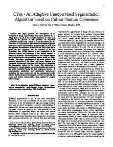
We have tried Hansen’s method of locating corners in L-curves. This involves smoothing the curve, fitting splines and then calculating the curvature. The convex corners show up as local maxima in the curvature. Hansen notes that using logarithms of ρ and η will tend to accentuate the corners. Unfortunately, we have had limited success with Hansen’s method (both with and without logarithms). The corners in our L-curves are not very distinct. The underlying problem is that in general different parts of the image can contain structures for which many λstable values are appropriate and as such the L-curve will contain many overlapped corners obscuring one-another. Our best results have been obtained by looking for convex corners in plots of log λ versus log ρ. An example is shown in Figure 1. Figure 1(f) shows the log λ versus log ρ curve with the only convex corner marked and Figure 1(e) is the segmentation corresponding to this choice of λ. We hope to pursue these ideas further in a future publication.
3 Results The performance of the four segmentation algorithms is shown in figure 1. From this simple test image, it can be seen that the full λ schedule algorithm produces a superior output in terms of the shape and number of the segmented areas. This is particularly evident in for example the bright inverted U-shaped region which the full λ-schedule has segmented as a single region, in contrast to the other three algorithms that have all over segmented the area. The superior performance of the new algorithm combined with its faster run-time makes it an attractive alternative.
4 Conclusion We have developed a fast and efficient algorithm for segmentation (based on [7]) with worst-case computational complexity of O(Nmax mn log2 mn), or even O(mn log2 mn) if there is an upper bound on the number of neighbours Nmax that is independent on image size. We have shown it to be superior to existing methods for segmenting SAR imagery.
5 Bibliography [1] M. Abramowitz and I. A. Stegun, Handbook of Mathematical Functions. New York, Dover, 1968. [2] R. Cook, I. McConnell, C. J. Oliver and E. Welbourne, “MUM (merge using moments) segmentation for SAR images,” Proceedings of the SPIE, 2316, pp. 92–103, 1994. [3] R. Cook, I. McConnell, D. Stewart and C. J. Oliver, “Segmentation and simulated annealing,” Proceedings of the SPIE, 2958, pp. 30–37, 1996. [4] T. H. Cormen, C. E. Leiserson and R. L. Rivest, Introduction to Algorithms. Cambridge, MA, MIT Press, 1992.
Proceedings of the 1999 Conference on Digital Image Computing: Techniques and Applications (DICTA-99), Perth. pp 35–41.
41
(a) Test
(b) RGW
(c) MUM 11.5
11
10.5
log ρ(λ)
10
9.5
9
8.5
8
7.5
7
6.5 −14
(d) Fitting
(e) Full λ Schedule
−12
−10
−8
log λ
−6
−4
−2
0
(f) Curve to Select λstop
Figure 1: The output of the various segmentation algorithms on a single SAR test image and (f) depicts the curve for the selection of λstop for optimum segmentation. (Acknowledgement: Image kindly supplied by NA Software).
[5] P. C. Hansen and D. P. O’Leary, “The use of the L-curve in the regularization of discrete ill-posed problems,” SIAM Journal of Scientific Computing, 14, no. 6, pp. 1487–1503, 1993. [6] R. M. Haralick and L. G. Shapiro, “Image segmentation techniques,” Computer Vision Graphics and Image Processing, 29, pp. 100–132, 1985. [7] G. Koepfler, C. Lopez and J. M. Morel, “A multiscale algorithm for image segmentation by variational methods,” SIAM Journal of Numerical Analysis, 31, no. 1, pp. 282–299, 1994. [8] J. -M. Morel and S. Solimini, Variational Methods in Image Segmentation. Boston, Birkh¨auser, 1995. [9] D. Mumford and J. Shah, “Boundary detection by minimizing functionals, I,” Proceedings of the IEEE Conference on Computer Vision and Pattern Recognition, pp. 22–26, 1985. [10] C. J. Oliver and S. Quegan, Understanding synthetic aperture radar images. Norwood, MA, Artech House, 1998. [11] C. J. Oliver, I. McConnell and D. Stewart, “Optimal texture segmentation of SAR clutter,” European Conference on Synthetic Aperture Radar, K¨onigswinter, Germany, pp. 81–84, Mar., 1996. [12] NA. Software, CAESAR Userguide Version 3.0 http://www.nasoftware.co.uk. Liverpool, UK, NA Software Limited, 1997. [13] R. G. White, “Change detection in SAR imagery,” International Journal of Remote Sensing, 12, no. 2, pp. 339–360, 1991.
Proceedings of the 1999 Conference on Digital Image Computing: Techniques and Applications (DICTA-99), Perth. pp 35–41.