Hindawi Publishing Corporation Advances in Mechanical Engineering Volume 2013, Article ID 456927, 10 pages http://dx.doi.org/10.1155/2013/456927
Research Article An Efficient and Accurate Method for Real-Time Processing of Light Stripe Images Xu Chen, Guangjun Zhang, and Junhua Sun Key Laboratory of Precision Opto-Mechatronics Technology, Ministry of Education, Beihang University, Beijing 100191, China Correspondence should be addressed to Junhua Sun;
[email protected] Received 8 July 2013; Revised 22 September 2013; Accepted 28 October 2013 Academic Editor: Liang-Chia Chen Copyright © 2013 Xu Chen et al. This is an open access article distributed under the Creative Commons Attribution License, which permits unrestricted use, distribution, and reproduction in any medium, provided the original work is properly cited. This paper describes a direction-guided method for real-time processing of light stripe images in practical active vision applications. The presented approach consists of three main steps. Firstly, we select two thresholds to divide the image into three classes, that is, the foreground, the background, and the undecided area. Then, we locate a feature point of the light stripe in the image foreground and calculate the local line direction at that point. Finally, we detect succeeding points along that direction in the foreground and the undecided area and directly exclude pixels which are in the normal direction of the line. We use synthetic and real images to verify the accuracy and efficiency of the proposed method. The experimental results show that the proposed algorithm gains a 1-fold speedup compared to the prevalent method without any loss of accuracy.
1. Introduction Due to the merit of the wide measurement range, noncontact capability, and high accuracy, active vision techniques have been widely used in fields of surface reconstruction, precision measurement, and industrial inspection [1, 2]. Nowadays, more and more vision systems for real-time measurement and inspection tasks have appeared [3]. Among the variety of active vision methods, line structured light vision technique is perhaps the most widespread. In this paper, we focus on the line structured light vision in real-time measurement applications. Light stripe processing plays an important role in line structured light vision applications in the following aspects. Firstly, the processing method should ensure the integrality of light stripes which are modulated by the surface of the object and contain the desired information. Secondly, the line point detection accuracy directly influences the measurement accuracy. Finally, the speed of the stripe processing algorithm is crucial in real-time applications. A time-consuming method is apparently not eligible for those tasks despite its high accuracy and robustness. To detect centric lines of curvilinear structures, there are many methods which can be roughly classified into two
categories. The first approach detects line points by only taking the gray values of the image into consideration and uses some local criteria such as extrema or centroids of gray values in a subregion [4, 5]. This kind of method is inclined to be affected by noisy pixels and the detection accuracy is relatively low. The second approach uses differential geometric properties to extract feature lines. These algorithms regard ridges and ravines in the image as the desired lines [6, 7]. Among those methods, the one proposed by Steger [8] is widely used in the community. Steger’s method firstly extracts line points by locally approximating the image function by its second order Taylor polynomial and determines the direction of the line at the current point from the Hessian matrix of the Taylor polynomial. After individual line points have been detected, a point linking algorithm is applied to facilitate further process. The linking step is necessary since we often want to get some characteristics about the feature line such as its length. Steger’s method has the advantages of high accuracy and nice robustness, whereas it also suffers from the drawback that the algorithm is computationally expensive, which is not sustainable in real-time applications. Based on Steger’s method, many revised algorithms aiming at processing light stripe images more efficiently have
2
Advances in Mechanical Engineering
(a) Wheel image with disturbing reflection lights
(b) Rail image with uneven light stripes
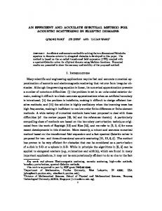
Figure 1: Real light stripe images affected by serious reflection.
been proposed. Hu et al. [9] utilize the separability of the Gaussian smoothing kernels and implement a recursive version of the Gaussian derivatives to approximate the original ones.Besides, Zhou et al. [10] present a composite processing method to detect the subpixel centers of light stripes based on region of interest (ROI). The method combines image thresholding with image dilation to automatically segment the ROIs of light stripes and then detects feature points in limited area. These algorithms have greatly improved the original Steger method, but it is still important to develop more efficient ones for real-time vision applications. In this paper, a direction-guided algorithm is given to accelerate the speed of line detection procedure. In the presented algorithm, the input light stripe image is firstly bilevel thresholded into image foreground, background, and the undecided area. Then, the first feature point of a new line in the light stripe is detected in the image foreground and the local line direction is calculated. Finally, succeeding line points are located in the foreground and undecided area along the direction and pixels which are in the normal direction of the line are excluded. Experiments on synthetic and real images have been conducted to verify the accuracy and efficiency of the proposed method and conclusions are drawn.
2. Bilevel Thresholding of the Light Stripe Image Most existing light stripe image processing methods can be divided into two stages, that is, image thresholding and line detection. Those methods assume that gray values of light stripes are markedly greater than those of the image background, and the threshold can be easily selected using Otsu’s method [11]. But the actual gray levels of light stripes may vary in a wide range and some stripe segments resemble the image background due to the serious reflection and large curvature of the object surface. In addition, some images may even be affected by serious disturbing lights which cannot be removed by optical filters. This circumstance occurs frequently when we try to recover profiles of some large scale metal parts whose surfaces are curving. Figure 1 exemplifies the aforementioned situation. Figure 1(a) is an image captured from a real freight wheel,
and Figure 1(b) is an image captured from a real train rail. We can see that there exists large area of disturbing lights in Figure 1(a), and the upper segments of light stripes in Figure 1(b) are relatively weaker than the lower parts. Given these conditions, thresholding simply using Otsu’s method may lead to the undesired results that some weak stripe segments are treated as the image background or the disturbing lights are seen as the foreground. To deal with light stripe images including those affected by serious reflection, we choose the bilevel thresholding strategy. That is, pixels with gray values greater than the higher threshold are treated as the foreground and those with gray values smaller than the lower threshold are seen as the background. Pixels with gray values which are between the two thresholds are treated as the undecided area. In the succeeding operations, we search the beginning feature point of a new line in the foreground and detect the potential points in the foreground and the undecided area. To determine the two thresholds, we combine the methods proposed by Otsu [11] and Rosin [12]. After calculating the image histogram, we can locate two gray values 𝑇min and 𝑇max which are corresponding to the highest peak and the last nonzero value of the histogram, respectively. Besides, gray levels 𝑇otsu and 𝑇rosin are selected using the methods proposed by Otsu and Rosin, respectively. We then determine the two thresholds 𝑇𝑙 and 𝑇ℎ according to the following rules: 𝑇𝑙 = 𝛼𝑇min + (1 − 𝛼) min {𝑇rosin , 𝑇otsu } 𝑇ℎ = 𝛽𝑇max + (1 − 𝛽) max {𝑇rosin , 𝑇otsu } , 𝛼 ∈ [0, 1] ,
(1)
𝛽 ∈ [0, 1] .
Actually, the parameters 𝛼 and 𝛽 are usually set as zeros for ordinary light stripe images. We only have to tune the two parameters when confronted with images which contain large area of disturbing reflection lights. Besides, we can utilize the entropy and the peak number of the histogram to decide whether the input image contains large area of disturbing reflection lights or not. Images with disturbing
Advances in Mechanical Engineering
3
lights often have larger entropies and more than two peaks in their histograms. The entropy calculation is given by
According to Steger’s conclusions, the parameter 𝜎 should satisfy the inequality
𝐿
𝐸 = − ∑ 𝑝𝑖 log 𝑝𝑖 .
𝜎≥
(2)
𝑖=0
Here, 𝑝𝑖 is the 𝑖th index of the normalized histogram ℎ(𝑡) and 𝐿 is the maximum gray value.
3. Determination of the First Feature Point of a New Line After bilevel thresholding the image into three classes, we can detect the first feature point of a new line by examining each unprocessed pixel in the image foreground using Steger’s method. In brief, if we denote the direction perpendicular to the line by 𝑛(𝑡), then the first directional derivative of the desired line point in the direction 𝑛(𝑡) should vanish and the second directional derivative should be of large absolute value. To compute the direction of the line locally for the image point to be processed, the first and second order partial derivatives 𝑟𝑥 , 𝑟𝑦 , 𝑟𝑥𝑥 , 𝑟𝑥𝑦 , and 𝑟𝑦𝑦 of the image pixel 𝑓(𝑥, 𝑦) have to be estimated by convolving it and its neighborhood points with the discrete two-dimensional Gaussian partial derivative kernels as follows:
𝐻 (𝑥, 𝑦) = (
(3)
𝑟𝑥𝑥 (𝑥, 𝑦) = 𝑓 (𝑥, 𝑦) ⊗ 𝑔𝑥𝑥 (𝑥, 𝑦) ,
𝑓 (𝑥0 + 𝑡𝑛𝑥 , 𝑦0 + 𝑡𝑛𝑦 ) = 𝑟 (𝑥0 , 𝑦0 ) + 𝑡𝑛𝑥 𝑟𝑥 (𝑥0 , 𝑦0 ) + 𝑡𝑛𝑦 𝑟𝑦 (𝑥0 , 𝑦0 ) 1 + 𝑡2 𝑛𝑥 𝑛𝑦 𝑟𝑥𝑦 (𝑥0 , 𝑦0 ) + 𝑡2 𝑛𝑥2 𝑟𝑥𝑥 (𝑥0 , 𝑦0 ) 2
(𝑝𝑥 , 𝑝𝑦 ) = (𝑡𝑛𝑥 , 𝑡𝑛𝑦 ) ,
𝑟𝑦𝑦 (𝑥, 𝑦) = 𝑓 (𝑥, 𝑦) ⊗ 𝑔𝑦𝑦 (𝑥, 𝑦) .
𝑡=−
𝑥2 + 𝑦2 1 𝑔 (𝑥, 𝑦) = exp (− ), 2𝜋𝜎2 2𝜎2
𝜕𝑔 (𝑥, 𝑦) 𝑥2 + 𝑦 2 𝑦 exp (− ), =− 𝜕𝑦 2𝜋𝜎4 2𝜎2 𝜕2 𝑔 (𝑥, 𝑦) 𝑥2 − 𝜎2 𝑥2 + 𝑦2 = exp (− ), 2 6 𝜕𝑥 2𝜋𝜎 2𝜎2
𝑔𝑦𝑦 (𝑥, 𝑦) =
𝜕2 𝑔 (𝑥, 𝑦) 𝑥2 + 𝑦2 𝑥𝑦 exp (− ), = 𝜕𝑥𝜕𝑦 2𝜋𝜎6 2𝜎2 2
𝑟𝑥 𝑛𝑥 + 𝑟𝑦 𝑛𝑦 𝑟𝑥𝑥 𝑛𝑥2 + 2𝑟𝑥𝑦 𝑛𝑥 𝑛𝑦 + 𝑟𝑦𝑦 𝑛𝑦2
.
(9)
Finally, the point (𝑥0 + 𝑝𝑥 , 𝑦0 + 𝑝𝑦 ) is declared a line point if (𝑝𝑥 , 𝑝𝑦 ) ∈ [−0.5, 0.5] × [−0.5, 0.5]. Using the aforesaid line point detection method, we can search the first feature point of a new line by examining every unprocessed pixel in the foreground. After detecting the first feature point, we can search succeeding line points and simultaneously exclude undesired pixels until no more line points exist in the current line. If there are no feature points left in the image foreground, the total processing procedure of the input light stripe image finishes.
𝜕𝑔 (𝑥, 𝑦) 𝑥2 + 𝑦2 𝑥 exp (− ), 𝑔𝑥 (𝑥, 𝑦) = =− 𝜕𝑥 2𝜋𝜎4 2𝜎2
2
(8)
where
The Gaussian kernels are given by
2
(7)
Thus, by setting the derivative of the Taylor polynomial along 𝑡 to zero, the subpixel point can be obtained:
𝑟𝑥𝑦 (𝑥, 𝑦) = 𝑓 (𝑥, 𝑦) ⊗ 𝑔𝑥𝑦 (𝑥, 𝑦) ,
2
(6)
1 + 𝑡2 𝑛𝑦2 𝑟𝑦𝑦 (𝑥0 , 𝑦0 ) . 2
𝑟𝑦 (𝑥, 𝑦) = 𝑓 (𝑥, 𝑦) ⊗ 𝑔𝑦 (𝑥, 𝑦) ,
𝑔𝑥𝑦 (𝑥, 𝑦) =
𝑟𝑥𝑥 𝑟𝑥𝑦 ). 𝑟𝑥𝑦 𝑟𝑦𝑦
The eigenvector corresponding to the eigenvalue of maximum absolute value is used as the normal direction 𝑛(𝑡) = (𝑛𝑥 , 𝑛𝑦 ) with ‖(𝑛𝑥 , 𝑛𝑦 )‖2 = 1. After determining the local normal direction, the Taylor polynomial of the image function at the pixel (𝑥0 , 𝑦0 ) along the direction (𝑛𝑥 , 𝑛𝑦 ) can be approximated by
𝑟𝑥 (𝑥, 𝑦) = 𝑓 (𝑥, 𝑦) ⊗ 𝑔𝑥 (𝑥, 𝑦) ,
𝑔𝑥𝑥 (𝑥, 𝑦) =
(5)
The parameter 𝑤 is defined as the half width of the light stripe in the image. Then the normal direction 𝑛(𝑡) can be determined by calculating the eigenvalues and eigenvectors of the Hessian matrix
𝑟 (𝑥, 𝑦) = 𝑓 (𝑥, 𝑦) ⊗ 𝑔 (𝑥, 𝑦) ,
𝑔𝑦 (𝑥, 𝑦) =
𝑤 . √3
4. Search of Potential Line Points and Exclusion of Undesired Pixels
2
𝜕 𝑔 (𝑥, 𝑦) 𝑦 − 𝜎 𝑥 +𝑦 = exp (− ). 2 6 𝜕𝑦 2𝜋𝜎 2𝜎2 (4)
Beyond the ROI-based techniques which exclude the operations on the image background, the proposed method utilizes
4
Advances in Mechanical Engineering
d1 p −n⊥
𝛽1
n1⊥ n2⊥
p1
𝛽2
n⊥ p2 d2 𝛼
(cx , cy )
Figure 2: Search of potential line points.
−n
p
n⊥
n Potential line points Undesired pixels
Figure 3: Exclusion of undesired pixels.
a further fact that the center line is only a little portion of the light stripe to be extracted. Therefore, it is unnecessary to process those undesired pixels around the feature points which are in the normal direction of the line. As a result, once we detect one feature point in the line, we can directly extract and link the succeeding points along the local direction of the line and then exclude pixels in the normal direction. It is the exclusion of undesired pixels that makes the presented method intrinsically gain great speedup when compared with other methods. Herein, we divide the light stripe extraction into two main steps: one is the search of potential line points and the other is the exclusion of undesired pixels. 4.1. Search of Potential Line Points. Starting from the first line point (𝑐𝑥 , 𝑐𝑦 ), we can directly search the succeeding points along both line directions 𝑛⊥ and −𝑛⊥ . In fact, we only have to process three neighboring pixels according to the current orientation of the line. We still use the feature point detection method described in Section 3 to determine whether a potential pixel is a line point or not. If there are two or more points found, we choose the one which minimizes the summation of the distance between the respective subpixel locations and the angle difference of the two points. Once a new line point is found, we update the local line direction. If there is no point eligible, we finish the search along the current direction and turn to the other direction. We end the line point linking until the searching operations along both directions finish and start to find a new line.
Figure 2 exemplifies the aforementioned directionguided line point searching step. As shown in the figure, the current orientation is assumed to be in the interval of [𝜋/8, 3𝜋/8], and the points (𝑐𝑥 + 1, 𝑐𝑦 − 1) and (𝑐𝑥 , 𝑐𝑦 − 1) are both found to be line points except for (𝑐𝑥 + 1, 𝑐𝑦 ). Then, the distances 𝑑1 , 𝑑2 and the angle differences 𝛽1 , 𝛽2 can be easily obtained. Suppose that 𝑑2 + 𝛽2 is smaller than 𝑑1 + 𝛽1 ; the point (𝑐𝑥 + 1, 𝑐𝑦 − 1) is then chosen as the new jumping-off point of the line, and the direction 𝑛2⊥ is regarded as the new orientation. 4.2. Exclusion of Undesired Pixels. Previous methods consider the light stripe extraction problem as two separated issues, that is, line point detection and feature point linking. Without exception, they first process all pixels in the region of interest, pick up the line points, and then link those points into lines. Actually, this kind of schemes often wastes calculations on pixels which are unnecessary to be processed, since it is only the central lines of light stripes that are the needed features in most cases. To avoid the unwanted line point detection operations on the undesired pixels, the proposed algorithm fuses the point detection and linking steps and utilizes the normal directions of detected points to exclude the pixels which are perpendicular to the line. Figure 3 illustrates the way of determining the undesired pixels. As shown in the figure, the three pixels with the red frame are the potential line points. Meanwhile, the fourteen pixels with the blue frame in both normal directions
Advances in Mechanical Engineering
5 Given input image I, get the two thresholds Tl and Th initializing the image mask Im (i, j) = 1, ∀i, j Update Im
Starting point c0 = (cx0 , cy0 ) which satisfies Im (cx0 , cy0 ) = 1, f(cx0 , cy0 ) > Th , and (px0 , py0 ) ∈ [−0.5, 0.5] exists?
No
Yes Succeeding point ci = (cxi , cyi ) which satisfies Im (cxi , cyi ) = 1, f(cxi , cyi ) > Tl , and
No
(pxi , pyi ) ∈ [−0.5, 0.5] exists?
Yes Link the succeeding point ci = (cxi , cyi ); exclude undesired pixels and update Im
Processing finishes
Figure 4: The flow chart of the proposed direction-guided approach.
𝑛 and −𝑛 are treated as undesired pixels and should be omitted. It is evident that the undesired pixels occupy the great mass of the light stripe, and thus it is significant to exclude them for the purpose of the speedup. 4.3. The Entire Direction-Guided Algorithm. Figure 4 summarizes the entire approach based on the idea of direction guidance. Note that starting points of feature lines are detected in the image foreground and potential line points are searched in the image foreground and undecided area.
5. Results and Discussion In order to demonstrate the accuracy and efficiency of the proposed method, experiments on synthetic and real images have been conducted, respectively. 5.1. Synthetic Image Data. To verify the accuracy of the line point detection, we manually generate an ideal image with one light stripe. The synthetic image shown in Figure 5(a) is 512 × 512, and the horizontal coordinate of the ideal center line of the light stripe is 256. After adding Gaussian white noise of 0 mean and 𝜎 standard deviation to the image, we use the presented method to detect line points and calculate the detection error 𝑒 by
𝑒=√
1 𝑁 2 ∑ 𝑥 − 𝑥̂𝑘 . 𝑁 𝑘=1 𝑘
(10)
Here, 𝑥𝑘 and 𝑥̂𝑘 are the ideal and detected position of the 𝑘th line point, respectively, and 𝑁 is the number of detected line points. Figure 5(b) is an example of the degraded image affected by Gaussian noise with 0 mean and 𝜎 = 0.4. We vary the noise level from 0.05 to 0.4. For each noise level, we perform 100 independent trials, and the results shown are the average. As we can see from Figure 5(c), errors increase linearly with the noise level. For 𝜎 = 0.4 (which is larger than the normal noise in practical situation), the detection error is less than 0.35. 5.2. Real Image Data. Here, we provide four representative examples to demonstrate the efficiency of the proposed method. All of those images are 960 × 700. Figure 6(a) is an image captured from a running train wheel using an exposure time of 50 us. Figure 6(b) is an image of a flat metal part with cross light stripes. Besides, Figure 6(c) is an image of a steel pipe with three light stripes and the image with five light stripes shown in Figure 6(d) is captured from a rail in use. Figure 7 displays the histograms of the example images and shows the positions of four important gray levels in green circles and two thresholds in red crosses. For all the test images, we directly use the gray level selected by Otsu’s method as the higher threshold. As for the lower threshold, we tune the parameter 𝛼 to be 0.75 for the wheel image affected by serious reflection lights and use the gray level selected by Rosin’s method as the lower threshold for other images. Figure 8 exhibits the bilevel thresholding results of the four images. From the thresholding results of the wheel and rail images, we can see that image thresholding merely utilizing Otsu’s method will mistake the weak segments of
6
Advances in Mechanical Engineering
(b) Degraded image with 𝜎 = 0.4
(a) The ideal image
0.35
0.3
The RMS error
0.25 0.2 0.15 0.1 0.05 0 0.05
0.1
0.15
0.2 0.25 𝜎: the noise level
0.3
0.35
0.4
(c) Errors versus the noise level
Figure 5: Accuracy verification experiment using a synthetic image.
light stripes for background just as expected. We can also observe that images are better segmented using bilevel thresholding especially for Figure 6(a). Figure 9 shows the line detection results. Although there may be several line points missing in the cross-sections of the light stripes due to the exclusion operations, the results are satisfying as a whole. To demonstrate the gain in speed, we compared the presented algorithm with those proposed by Steger [8] and Zhou et al. [10]. The experiments were conducted on an Intel Core2 2.93 GHz machine running Windows 7 and the three algorithms were implemented under the Visual Studio 2012 environment. For every test image, experiments were repeated 100 times under the same conditions and a comparison of mean running time is shown in Table 1. From the table, we can see that the time consumed by the proposed method is less than
Table 1: Comparison of mean running time of different line detection methods (ms). Images Figure 6(a) Figure 6(b) Figure 6(c) Figure 6(d)
Steger 265 254 255 256
Zhou 45 39 42 41
Proposed 15 18 25 22
half of the time consumed by Zhou’s method and about tenth of the time consumed by Steger’s method. Furthermore, the excluded pixels of the test images during processing are shown in Figure 10 with black brush to illustrate the effect of the exclusion operations of undesired pixels and visually explain the speedup of the proposed
Advances in Mechanical Engineering
7
(a) Two lines
(b) Cross lines
(c) Three lines
(d) Five lines
Figure 6: Real example images to verify the efficiency.
0.09
0.7
Tmin = 5
0.08
0.5
0.06
Frequency
Frequency
0.07
Tl = 10
0.05 0.04 0.03 0.02
Trosin = 25
0.01 0
Tmin = 3
0.6
Th = Totsu = 97 0
50
100
200
0.3 0.2 0.1
Tmax = 255 150
0.4
0
250
Tl = Trosin = 6 0
50
Gray level
Frequency
Frequency
150
200
250
(b)
Th = Totsu = 121 100
100
Tmax = 255 2 5 25
Gray level
(a) 0.5 Tmin = 2 0.45 0.4 0.35 0.3 0.25 0.2 0.15 0.1 0.05 Tl = Trosin = 7 0 0 50
Th = Totsu = 124
150
Gray level
Tmax = 255 200
250
0.9 Tmin = 0 0.8 0.7 0.6 0.5 0.4 0.3 0.2 0.1 Tl = Trosin = 3 Th = Totsu = 78 0 0 50 100 150 Gray level
(c)
(d)
Figure 7: Selected thresholds for test images.
Tmax = 253 200
250
8
Advances in Mechanical Engineering
(a)
(b)
(c)
(d)
Figure 8: Bilevel thresholding results of test images.
(a)
(b)
(c)
(d)
Figure 9: Line detection results of test images.
Advances in Mechanical Engineering
9
(a) Excluded pixels of Figure 6(a)
(b) Excluded pixels of Figure 6(b)
(c) Excluded pixels of Figure 6(c)
(d) Excluded pixels of Figure 6(d)
Figure 10: Excluded pixels of the test images during processing.
algorithm. It is noticeable that most of the undesired pixels around the line points are excluded during the line detection process, and thus a lot of unnecessary calculations are eliminated in advance.
Acknowledgment
6. Conclusion
References
A direction-guided light stripe processing approach is presented. This method is characterized by its sound utilization of the local orientations of light stripes and has the following advantages. Firstly, the proposed method utilizes a bilevel thresholding method which not only ensures the integrality of uneven light stripes but also avoids blind calculations on undecided pixels. Secondly, the method retains the high accuracy of line point detection, since the point extraction algorithm is the same as the state-of-the-art one. Thirdly, the point detection and linking steps are combined tightly, and thus it is more flexible to do some specific operations such as selective processing without the need of extracting all the line points. Finally, the exclusion operations of undesired pixels successfully avoid a mass of unwanted calculations and bring a remarkable speedup. Although there may be several feature points missing when dealing with cross light stripes due to the exclusion operation, the data loss is extremely limited. As a whole, the proposed method may be more suitable to be applied in real-time structured light vision applications considering its high accuracy and great efficiency.
[1] P. Lavoie, D. Ionescu, and E. M. Petriu, “3-D object model recovery from 2-D images using structured light,” IEEE Transactions on Instrumentation and Measurement, vol. 53, no. 2, pp. 437– 443, 2004. [2] Z. Liu, J. Sun, H. Wang, and G. Zhang, “Simple and fast rail wear measurement method based on structured light,” Optics and Lasers in Engineering, vol. 49, no. 11, pp. 1343–1351, 2011. [3] J. Xu, B. Gao, J. Han et al., “Realtime 3D profile measurement by using the composite pattern based on the binary stripe pattern,” Optics & Laser Technology, vol. 44, no. 3, pp. 587–593, 2012. [4] D. Geman and B. Jedynak, “An active testing model for tracking roads in satellite images,” IEEE Transactions on Pattern Analysis and Machine Intelligence, vol. 18, no. 1, pp. 1–14, 1996. [5] M. A. Fischler, “The perception of linear structure: a generic linker,” in Proceedings of the 23rd Image Understanding Workshop, pp. 1565–1579, Morgan Kaufmann Publishers, Monterey, Calif, USA, 1994. [6] D. Eberly, R. Gardner, B. Morse, S. Pizer, and C. Scharlach, “Ridges for image analysis,” Tech. Rep. TR93-055, Department of Computer Science, University of North Carolina, Chapel Hill, NC, USA, 1993.
This work is supported by the National Natural Science Foundation of China under Grant nos. 61127009 and 61275162.
10 [7] A. Busch, “A common framework for the extraction of lines and edges,” International Archives of the Photogrammetry and Remote Sensing, vol. 31, part B3, pp. 88–93, 1996. [8] C. Steger, “An unbiased detector of curvilinear structures,” IEEE Transactions on Pattern Analysis and Machine Intelligence, vol. 20, no. 2, pp. 113–125, 1998. [9] K. Hu, F. Zhou, and G. Zhang, “Fast extrication method for sub-pixel center of structured light stripe,” Chinese Journal of Scientific Instrument, vol. 27, no. 10, pp. 1326–1329, 2006. [10] F.-Q. Zhou, Q. Chen, and G.-J. Zhang, “Composite image processing for center extraction of structured light stripe,” Journal of Optoelectronics.Laser, vol. 19, no. 11, pp. 1534–1537, 2008. [11] N. Otsu, “A threshold selection method from gray-level histograms,” IEEE Transactions on Systems, Man, and Cybernetics, vol. 9, no. 1, pp. 62–66, 1979. [12] P. L. Rosin, “Unimodal thresholding,” Pattern Recognition, vol. 34, no. 11, pp. 2083–2096, 2001.
Advances in Mechanical Engineering