Given a belief network with evidence, the task of finding the l most probable ex planations (MPE) in the belief network is that of identifying and ordering the l most.
342
Li and D'Ambrosio
An efficient approach for finding the MPE in belief networks
Zhaoyu Li
Department of Computer Science Oregon State University Corvallis, OR 97331
Abstract
Given a belief network with evidence, the task of finding the l most probable ex planations (MPE) in the belief network is that of identifying and ordering the l most probable instantiations of the non-evidence nodes of the belief network. Although many approaches have been proposed for solving this problem, most work only for restricted topologies (i.e., singly connected belief net works). In this paper, we will present a new approach for finding l MPEs in an arbitrary belief network. First, we will present an al gorithm for finding the MPE in a belief net work. Then, we will present a linear time al gorithm for finding the next MPE after find ing the first MPE. And finally, we will discuss the problem of finding the MPE for a subset of variables of a belief network, and show that the problem can be efficiently solved by this approach. 1
Introduction
Finding the Most Probable Explanation(MPE) [21] of a set of evidence in a Bayesian (or belief) network is the identification of an instantiation or a composite hypothesis of all nodes except the observed nodes in the belief network, such that the instantiation has the largest posterior probability. Since the MPE provides the most probable states of a system, this technique can be applied to system analysis and diagnosis. Find ing the 1 most probable explanations of some given evidence is to identify the 1 instantiations with the 1 largest probabilities. There have been some research efforts for finding MPE in recent years and several methods have been pro posed for solving the problem. These previously devel oped methods can roughly be classified into two differ ent groups. One group of methods consider the MPE as the problem of minimal-cost-proofs which works for finding the best explanation for text [11, 2, 31].
Bruce D'Ambrosio
Department of Computer Science Oregon State University Corvallis, OR 97331
In finding the minimal-cost-proofs, a belief network is converted to Weighted Boolean Function Directed Acyclic Graphs (WBFDAG) [31], or cost-based ab duction problems, and then the best-search techniques are applied to find MPE in the WBFDAGs. Since the number of the nodes in the converted graph is expo nential in the size of the original belief network, effi ciency of this technique seems not comparable with some algorithms directly evaluating belief networks [1]. An improvement is to translate the minimal-cost proof problems into 0-1 programming problems, and solve them by using simplex combined with branch and bound techniques (24, 25, 1]. Although the new tech nique outperformed the best-first search technique, there are some limitations for using it, such as that the original belief networks should be small and their structures are close to and-or dags. The second group of methods directly evaluate belief networks for find ing the MPE but restrict the type of belief networks to singly connected belief networks [21, 33, 34] or a particular type of belief networks such as BN20 [9], bipartite graphs [36]. Arbitrary multiply connected belief networks must be converted to singly connected networks and then are solved by these methods. The algorithm developed by J. Pearl [21] presents a mes sage passing technique for finding two most probable explanations; but this technique is limited to only find ing two explanations [17] and can not be applied to multiply connected belief networks. Based on the mes sage passing technique, another algorithm [33, 34] has been developed for finding 1 most probable explana tions. Although this algorithm has some advantages over the previous one, it is also limited to singly con nected belief networks. In this paper, we will present an approach for finding the 1 MPEs for arbitrary belief networks. First we will present an algorithm for finding the MPE. Then, we will present a linear time algorithm for finding the next MPE; so the 1 MPEs can be efficiently found by a�tivating the algorithm l 1 times. Finally, we will d1scuss the problem of finding the MPE for a subset of variables in belief networks, and present an algorithm to solve this problem. -
The rest of the paper is organized as follows. Section
An efficient approach for finding the MPE in belief networks
2 present an algorithm for finding the MPE. Section 3 presents a linear time algorithm for finding the next MPE after finding the first MPE. Section 4 discusses the problem of finding the MPE for a subset of vari ables of a belief network. And finally, section 5 sum marizes the research. 2
The algorithm for finding the MPE
There are two basic operations needed for finding the MPE: comparison for choosing proper instantiations and multiplication for calculating the value of the MPE. The difficulty of the problem of finding the MPE lies in finding or searching the right instantiations of all variables in a belief network since the multiplica tions for the MPE is simply given right instantiation of all variables. This means that finding the MPE can be a search problem. We can use search with back tracking techniques to find the MPE, but it may not be an efficient way because the search complexity is exponential with respect to the number of variables of a belief network in worst case. We proposed a non-search method for finding the MPE. If we know the full joint probability of a belief network, we can obtain the I MPEs by sorting the joint probability table in descending order and choosing the first I instantiations. However, computing the full joint probability is quite inefficient. An improvement of the method is to use the "divide and conquer" technique. We can compute a joint probability distribution of some of distributions, llind the largest instantiations of some variables in the distribution and eliminate those variables from the distribution; then, we com bine the partially instantiated distribution with some other distributions until all distributions are combined together. In a belief network, if a node has no descendants, we can find the largest instantiations of the node from its conditional distribution to support the MPE. In general, if some variables only appear in one distribu tion, we can obtain the largest instantiations of these variables to support the MPE. When a variable is in stantiated in a distribution, the distribution is reduced and doesn't contain the variable; but each item of the reduced distribution is constrained by the instantiated value of that variable. Given distributions of an arbitrary belief network, the algorithm for finding the MPE is: 1. For any node x having no descendants, reduce its conditional distribution by choosing the largest instantiated values of the node for each instantia tion of the other variables. The reduced distribu tion has no variable x in it. 2. Create a factoring for combining all distributions; 3. Combine these distributions according to the fac toring. If a result distribution of a conformal product (i.e. the product of two distributions)
343
contains a variable x which doesn't appear in any other distribution, reduce the result distribution (as in step 1), so that the reduced distribution doesn't contain variable x in it. The largest instantiated value of the last result distri bution is the MPE1. Figure 1 is a simple belief network example to illus trate the algorithm. Given the belief network in fig ure 1, we want to compute its MPE. There are six distributions in the belief network. We use D(x,y) to denote a distribution with variables x and y in it and d(x = 1, y = 1) to denote one of items of the D(x,y). In the step 1 of the algorithm, the distributions rele vant to nodes e and f are reduced. For instance, p(fid) becomes D(d): d(d = 0) = 0. 7 with f = 1; d(d = 1) = 0.8 with f = 0. In step 2 a factoring should be created for these dis tributions. For this example we assume the factoring IS:
(((D(a)* D(a,c))*(D(b)*D(a,b,d)))*(D(c,d)*D(d))). In step 3, these distributions are combined together some combined distributions are reduced if possible. The final combined distribution is D(c, d): d(c = 1, d = 1) = .0224 with a = 1 b = 0 e = 1 f = 0; d(c = 1, d = 0) = .0753 with a = 0 b = 0 e = 1 I == 1; d(c = 0, d = 1) = .0403 with a = 0 b = 1 e = 1 f = 0; d(c = 0, d = 0) = .1537 with a = 0 b = 0 e = 0 I= 1. Choosing the largest instantiation of D(c,d), the MPE is: p(a = O,b = O,c = O,d = O,e = 0,1 = 1). If an unary operator ., is defined for a probability distri bution p(yix), .,p(yix), to indicate the operation of instantiating the variable x and eliminating the vari able from the distribution p(yix), the computations above for finding the MPE can be represented as: cl>c,d(cl>a((p(a) * p(a, c)) * cl>b(p(b) * p(a,b,d))) *(ep(eic,d) * Jp{fld))). The most time consuming step in the algorithm is step 3. In step 1, the comparisons needed for instantiating a variable of a distribution is exponential in the num ber of conditioning variables of that variable. This cost is determined by the structure of a belief net work. Factoring in step 2 could be arbitrary. In step 3, total computational cost consists of multiplications for combining distributions and comparisons for in stantiating some variables in some intermediate result distributions. The number of variables of a conformal product or an intermediate result distribution is usu ally great than the that of distributions in step 1. If we use the maximum dimensionality to denote the max imum number of variables in conformal products, the time complexity of the algorithm is exponential with respect to the maximum dimensionality. 1 Step 2 and step 3 can be mixed together by finding a partial factoring for some distributions and combining them.
344
Li and D'Ambrosio
p(a): p(a=l)=0.2 p(b): p(b=1)=0.3 p(cla): p(c=lla=1)=0.8 p(c=lla=0)=0.3 p(dla,b): p(d=lla=l,b=1)=0.7 p(d=lla=l,b=0)=0.5 p(d=lla=O,b=l)=0.5 p(d=lla=O,b=0)=0.2 p(elc,d): p(e=llc=l,d=l)=0.5 p(e=llc=l,d=0)=0.8 p(e=llc=O,d=l)=0.6 p(e=llc=O,d=0)=0.3 p(fld): p(f=lld=1)=0.2 p(f=lld=0)=0.7 Figure 1: A simple belief network. Step 2 is important to the efficiency of the algorithm because the factoring determines the maximum dimen sionality of conformal products, namely the time com plexity of the algorithm. Therefore, we consider the problem of efficiently finding the MPE as a factoring problem. We have formally defined an optimization problem, optimal factoring [16], for handling the fac toring problem. We have presented an optimal fac toring algorithm with linear time cost in the number of nodes of a belief network for singly connected belief networks, and an efficient heuristic factoring algorithm with polynomial time cost for multiply connected be lief networks [16]. For reason of paper length, the opti mal factoring problem will not be discussed here. The purpose of proposing the optimal factoring problem is that we want to apply some techniques developed in the field of combinatorial optimization to the optimal factoring problem, and apply the results from the op timal factoring problem to speedup the computation for finding the MPE. It should be noticed that step 2 of the algorithm is a process of symbolic reasoning, having nothing to do with probability computation. There is a trade-off be-: tween the symbolic reasoning and probability compu tation. We want to use the polynomial time cost of this symbolic reasoning process to reduce the exponential time cost of the probability computation. 3
Finding the l MPEs in belief networks
In this section, we will show that the algorithm pre sented in section 2 provides an efficient basis for finding the 1 MPEs. We will present a linear time algorithm for finding next MPE. The I MPEs can be obtained by first finding the MPE and then calling the linear algorithm l - 1 times to obtain next 1 - 1 MPEs.
3.1
Sources of the next MPE
Having found the first MPE, we know the instantiated value of each variable and the associated instantiations of the other variables in the distribution in which the variable was reduced. It is obvious that the instanti ated value is the largest value of all instantiations of the variable with the same associated instantiations for the other variables in the distribution. If we replace that value with the second largest instantiation of the variable at the same associated instantiations of the other variables in the distribution, the result should be one of candidates for the second MPE. For example, if d(a = A1, b = B1, ... ,g = Gt) is the instantiated value for the first MPE when the variable a is instantiated, the value d( a = A1, b = Bt, ... , g = G1) is the largest instantiation of the variable a with b = B1, ... ,g = G1. If we replace d(a = A1, b = B1, ... , g = GI) with d(a = A2, b = B11 ... ,g = Gt), the second largest instantiation of a given the same instantiation of B through G, and re-evaluate all nodes on the path from that reduction operation to the root of the factor tree, the result is one of the candidates for the second MPE. The total set of candidates for the second MPE comes from two sources. One is the second largest value of the last conformal product in finding the first MPE; and the other is the largest value of instantiations com puted in the same computation procedure as for find ing the first MPE but replacing the largest instantia tion of each variable independently where it is reduced with the second largest instantiation. The similar idea can be applied for finding the third MPE, and so on. The factoring (or the evaluation tree) generated in step 2 of the algorithm in section 2 provides a structure for computing those candidates. We use the example in that section to illustrate the process. Figure 2 is the evaluation tree for finding the MPE for the belief network in figure 1 section 2. Leaf-nodes
An efficient approach for finding the MPE in belief networks
345
()) c,d
I