Incremental Sigmoid Belief Networks for Grammar Learning

Journal of Machine Learning Research 11 (2010) 3541-3570

Submitted 4/10; Revised 10/10; Published 12/10

Incremental Sigmoid Belief Networks for Grammar Learning James Henderson

JAMES . HENDERSON @ UNIGE . CH

Department of Computer Science University of Geneva 7 route de Drize, Battelle bâtiment A 1227, Carouge, Switzerland

Ivan Titov

TITOV @ MMCI . UNI - SAARLAND . DE

MMCI Cluster of Excellence Saarland University Saarbrücken, Germany

Editor: Mark Johnson

Abstract We propose a class of Bayesian networks appropriate for structured prediction problems where the Bayesian network’s model structure is a function of the predicted output structure. These incremental sigmoid belief networks (ISBNs) make decoding possible because inference with partial output structures does not require summing over the unboundedly many compatible model structures, due to their directed edges and incrementally specified model structure. ISBNs are specifically targeted at challenging structured prediction problems such as natural language parsing, where learning the domain’s complex statistical dependencies benefits from large numbers of latent variables. While exact inference in ISBNs with large numbers of latent variables is not tractable, we propose two efficient approximations. First, we demonstrate that a previous neural network parsing model can be viewed as a coarse mean-field approximation to inference with ISBNs. We then derive a more accurate but still tractable variational approximation, which proves effective in artificial experiments. We compare the effectiveness of these models on a benchmark natural language parsing task, where they achieve accuracy competitive with the state-of-the-art. The model which is a closer approximation to an ISBN has better parsing accuracy, suggesting that ISBNs are an appropriate abstract model of natural language grammar learning. Keywords: Bayesian networks, dynamic Bayesian networks, grammar learning, natural language parsing, neural networks

1. Introduction In recent years, there has been increasing interest in structured prediction problems, that is, classification problems with a large (or infinite) structured set of output categories. The set of output categories are structured in the sense that useful generalisations exist across categories, as usually reflected in a structured representation of the individual categories. For example, the output categories might be represented as arbitrarily long sequences of labels, reflecting generalisations across categories which share similar sets of sub-sequences. Often, given an input, the structure of the possible output categories can be uniquely determined by the structure of the input. For example in sequence labelling tasks, all possible output categories are label sequences of the same length as the input sequence to be labelled. In this article, we investigate structured classification problems c

2010 James Henderson and Ivan Titov.

H ENDERSON AND T ITOV

where this is not true; the structure of the possible output categories is not uniquely determined by the input to be classified. The most common type of such problems is when the input is a sequence and the output is a more complex structure, such as a tree. In reference to this case, we will refer to problems where the output structure is not uniquely determined by the input as “parsing problems”. Such problems frequently arise in natural language processing (e.g., prediction of a phrase structure tree given a sentence), biology (e.g., protein structure prediction), chemistry, or image processing. We will focus on the first of these examples, natural language parsing. The literature on such problems clearly indicates that good accuracy cannot be achieved without models which capture the generalisations which are only reflected in the output structure. For example, in English sentences, if a noun is parsed as the subject of a verb, then these words must be compatible in their singular/plural markings, independent of whether they are near each other in the input sentence. In addition to limiting the scope of this article to parsing problems, we focus on tasks where the training data specifies the output structure, but the labelling of this structure is not fully annotated. While the unannotated labelling may not be evaluated in the task, by assuming incomplete labelling we allow our models to capture generalisation which are not directly reflected in the labelled output structure given for training. For example, the training data for natural language parsing problems is generally assumed to be a tree, but assuming that all generalisations can be expressed in terms of one-level fragments of the tree leads to poor empirical performance. However, much better performance can be achieved with such a model by extending the labelling to include features of the structural context (Charniak, 2000). Because we want to learn the necessary additional labelling, we need to solve a limited form of grammar induction. Graphical models provide the formal mechanisms needed to learn and reason about incomplete labelling, using latent variables. They also provide the formal mechanisms needed to specify the statistical dependencies implied by the structure of a single output category. However, these mechanisms are not sufficient to specify a complete probability model for a parsing problem, because we need to specify the statistical dependencies for the complete space of possible output categories. As we will discuss in Section 3, even graphical models for unbounded sequence labelling, such as dynamic Bayesian networks, are in general not adequate for this task, because they are limited to finite-state models. There are well established methods for specifying probabilistic models of parsing problems, based on grammar formalisms, such as probabilistic context-free grammars (PCFGs). The grammar formalism defines how the complete space of possible pairs of an input sequence with an output structure can be specified as a set of sequences of decisions about the input-output pair. Each possible sequence of decisions, called a derivation, specifies a single input-output pair (e.g., phrase structure tree or protein structure). The probability model is then defined in terms of probabilities for each decision. In its most general form, these decision probabilities are conditioned on anything from the unbounded history of previous decisions: P(T ) = P(D1 , ..., Dm ) = ∏ P(Dt |D1 , . . . , Dt−1 ),

(1)

t

where T is the input-output structure and D1 , . . . , Dm is its equivalent sequence of decisions. In PCFGs, the context-free assumption means that only a bounded amount of the history D1 , . . . , Dt−1 is relevant to the probability for decision Dt . The context-free assumption only allows statistical dependencies within each bounded one-level subtree of the output tree, so two such subtrees can only interact through the bounded choice of label for the node they share, if any. Because the context-free assumption is defined in terms of the output structure, not in terms of the 3542

I NCREMENTAL S IGMOID B ELIEF N ETWORKS

input sequence, which decisions in the history are relevant depends on the output structure specified by the derivation. In graphical models, such a specification of which decisions are statistically dependent on which other decisions is called the “model structure”. Thus PCFGs, like other grammar formalisms, are examples of models where the model structure is a function of the output structure, not just of the input sequence. This is the fundamental distinction between models of parsing problems and models of sequence labelling problems, and it will be central to our discussions in this article. The most common approach to building probability models for parsing problems is to use PCFGs without any latent variables (e.g., Charniak, 2000; Collins, 1999; Durbin et al., 1998), but this approach relies on hand-built sets of features to represent the unbounded decision histories in (1). Latent probabilistic context-free grammars (LPCFGs) (Matsuzaki et al., 2005) extend the node labels of PCFGs with latent annotations, but previous proposals have successfully induced only a small number of latent annotations. An alternative proposal to extending the labelling of parse trees is to use the hidden units of a neural network (Henderson, 2003). In the model of Henderson (2003), vectors of hidden unit values decorate the positions t in the derivation sequence, and are used to encode features of the unbounded derivation history D1 , . . . , Dt−1 . As with LPCFGs, the pattern of interdependencies between layers of hidden units is a function of the output structure, making it appropriate for parsing problems. But unlike LPCFGs, the pattern of interdependencies is not required to respect the context-free assumption. This model achieved state-of-the-art results, but there is no clear probabilistic semantics for the induced hidden representations. In this article, we propose a class of graphical models which we call incremental sigmoid belief networks (ISBNs), which are closely related to the neural network of Henderson (2003), but which have a clear probabilistic semantics for all their variables. ISBNs are a kind of sigmoid belief network (Neal, 1992), but are dynamic models and have an incrementally specified set of statistical dependencies. Each position in the decision sequence has a vector of latent state variables, which are statistically dependent on variables from previous positions via a pattern of edges determined by the previous decisions. This incrementally specified model structure allows ISBNs to capture the generalisations which are only reflected in the output structure, such as the tendency towards correlations which are local in the output structure, which motivates the context-free assumption of PCFGs. Allowing the model structure to depend on the output structure means that the complete model structure is not known until the complete output derivation is known. In general, this can complicate decoding (i.e., parsing) because computing probabilities for sub-derivations requires marginalising out the unknown portion of the model structure, which in the worst case could require summing over an unbounded number of possible model structures. The properties of ISBNs avoid this problem because the probability of a derivation prefix is always independent of the unknown portion of the model structure, as discussed in Section 3. Despite this simplification, exact inference (i.e., computing probabilities) is not in general tractable in ISBNs, because they allow large vectors of latent variables in a heavily interconnected directed model. We demonstrate the practical applicability of ISBN models by providing efficient approximate inference methods. We consider two forms of approximation for ISBNs, a feed-forward neural network approximation (NN) and a form of mean field approximation (Saul and Jordan, 1999). In Section 5, we first show that the neural network model in Henderson (2003) can be viewed as a coarse approximation to inference with ISBNs. We then propose an incremental 3543


mean field method (IMF), which provides an improved approximation but remains tractable. Both these approximations give us valid probability models. In Section 7, we present two empirical evaluations. In the first experiment, we trained both of the approximation models on artificial data generated from random ISBNs. The NN model achieves a 60% average relative error reduction over a baseline model and the IMF model achieves a further 27% average relative error reduction over the NN model. These results demonstrate that the distribution of output structures specified by an ISBN can be approximated, that these approximations can be learnt from data, and that the IMF approximation is indeed better than the NN approximation. In the second experiment, we apply both of the approximation models to phrase structure parsing with data from the Wall Street Journal Penn Treebank (Marcus et al., 1993). The IMF model achieves statistically significant error reduction of about 8% over the NN model. Results of the IMF model are non-significantly worse (less than 1% relative error increase) than the results of one of the best known history-based models of parsing (Charniak, 2000). We argue that this correlation between better approximation and better accuracy suggests that ISBNs are a good abstract model for structured prediction. Section 8 discusses related work not covered in the rest of this article. It focuses particularly on previous work on LPCFGs.

2. Inference with Sigmoid Belief Networks Before defining ISBNs, we provide background on sigmoid belief networks. A sigmoid belief network (SBN) (Neal, 1992) is a type of Bayesian network. Bayesian networks are directed acyclic graphs where the nodes are variables and the edges specify statistical dependencies between variables. SBNs have binary variables which have conditional probability distributions (CPDs) of the form: P(Si = 1|Par(Si )) = σ(

∑

Ji j S j ),

(2)

S j ∈Par(Si )

where Par(Si ) is the set of variables with edges directed to Si , σ denotes the logistic sigmoid function σ(x) = 1/(1 + e−x ), and Ji j is the weight for the edge from variable S j to variable Si .1 SBNs are similar to feed-forward neural networks, but unlike neural networks, SBNs have a precise probabilistic semantics of their hidden variables. In ISBNs we consider a generalised version of SBNs where we allow variables with any range of discrete values. The normalised exponential function is used to define the CPDs at these nodes:

P(Si = k|Par(Si )) =

exp(∑S j ∈Par(Si ) Wki j S j ) ∑k′ exp(∑S j ∈Par(Si ) Wki′ j S j )

,

(3)

where W i is the weight matrix for the variable Si . Exact inference with all but very small SBNs is not tractable. Initially sampling methods were used (Neal, 1992), but they are also not feasible for large networks, especially for the dynamic models of the type described in Section 4. Variational methods have also been proposed for approximating SBNs (Saul et al., 1996; Saul and Jordan, 1999). The main idea of variational methods (Jordan 1. For convenience, where possible, we will not explicitly include bias terms in expressions, assuming that every latent variable in the model has an auxiliary parent variable set to 1.

3544


et al., 1999) is, roughly, to construct a tractable approximate model with a number of free parameters. The free parameters are set so that the resulting approximate model is as close as possible to the original model for a given inference problem. The simplest example of a variational method is the mean field method, originally introduced in statistical mechanics and later applied to neural networks in Hinton et al. (1995). Let us denote the set of visible variables in the model by V and latent (hidden) variables by H = h1 , . . . , hl . The mean field method uses a fully factorised distribution Q(H|V ) = ∏i Qi (hi |V ) as the approximate model, where each Qi is the distribution of an individual latent variable. The independence between the variables hi in this approximate distribution Q does not imply independence of the free parameters which define the Qi . These parameters are set to minimise the Kullback-Leibler divergence between the approximate distribution Q(H|V ) and the true distribution P(H|V ) or, equivalently, to maximise: LV = ∑ Q(H|V ) ln H

P(H,V ) . Q(H|V )

(4)

The expression LV is a lower bound on the log-likelihood ln P(V ). It is used in the mean field theory (Saul and Jordan, 1999) as an approximation of the log-likelihood. However, in our case of dynamic graphical models, as explained later, we have to use a different approach which allows us to construct an incremental structured prediction method without needing to introduce the additional parameters proposed in Saul and Jordan (1999), as we will discuss in Section 5.3.

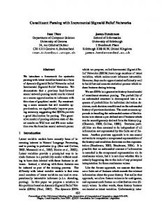
3. Incrementally Specifying Model Structure We want to extend SBNs to make them appropriate for modelling parsing problems. As discussed in the introduction, this requires being able to model arbitrarily long decision sequences D1 , ..., Dm , and being able to specify the pattern of edges (the model structure) as a function of the chosen output structure. In this section, we define how incremental sigmoid belief networks specify such model structures. To extend SBNs for processing arbitrarily long sequences, such as the derivation decision sequence D1 , ..., Dm , we use dynamic models. This gives us a form of dynamic Bayesian network (DBN). To handle unboundedly long sequences, DBNs specify a Bayesian network template which gets instantiated for each position in the sequence, thereby constructing a Bayesian network which is as large as the sequence is long. This constructed Bayesian network is illustrated in the rightmost graph of Figure 1, where the repeated two-box pattern is the template, and the left-to-right order is the derivation order. This template instantiation defines a new set of variables for each position in the sequence, but the set of edges and parameters for these variables are the same as in other positions. The edges which connect variables instantiated for different positions must be directed forward in the sequence, thereby allowing a temporal interpretation of the sequence. DBNs based on sigmoid belief networks were considered in Sallans (2002) in the context of reinforcement learning. Normally, DBNs only allow edges between adjacent (or a bounded window of) positions, which imposes a Markov assumption on statistical dependencies in the Bayesian network. The problem with only allowing edges between variables instantiated at positions which are adjacent (or local) in the decision sequence is that this does not allow the model structure to adequately reflect the correlations found in parsing problems. In particular, in many domains, correlations tend to be local in the output structure, even when they are not local in the derivation sequence for that structure. To capture these correlations in the statistical dependencies learnt by the model, we want 3545


ROOT

ROOT

ROOT S

ROOT

S

NP

NP

Mary

VP

runs Mary

Mary

ROOT

runs

S

ROOT NP

VP

NP

Mary runs

Mary ROOT

ROOT

S

S NP Mary

NP VP Mary runs

Figure 1: Illustration of the predictive LR derivation of an output structure and its associated incremental specification of an ISBN model structure (ordered top-to-bottom, left-to-right). Dotted lines indicate the top of the parser’s stack at each derivation decision in the model structure.

the edges of the model to reflect locality in the output structure. This requires specifying edges based on the actual outputs in the decision sequence D1 , ..., Dm , not just based on adjacency in this sequence. ′ We constrain this edge specification so that a decision Dt can only effect the placement of ′ edges whose destination variable is at a position t > t ′ after the decision Dt . This gives us a form of switching model (Murphy, 2002), where each decision switches the model structure used for the remaining decisions. We allow the incoming edges for a given position to be any discrete function of the sequence of decisions which precede that position. For this reason, we call our model an “incremental” model, not just a dynamic model; the structure of the Bayesian network is determined incrementally as the decision sequence proceeds. This incremental specification of the model structure is illustrated in Figure 1 (the directed graphs), along with the partial output structures incrementally specified by the derivation (the trees). In Figure 1, dotted lines associate a position’s instantiated template with the node in the output structure which is on top of the parser’s stack when making that position’s decision. Note that the incoming edges for a position’s instantiated template reflect edges between the associated nodes in the partial output structure. Any discrete function can be used to map the preceding sequence of decisions to a set of incoming edges for a given decision. In general, we can characterise this function in terms of an automaton which reads derivations and deterministically outputs model structures. For every derivation prefix D1 , ..., Dt−1 , the automaton outputs a set of labelled positions in the derivation prefix. For each labelled position (t − c, r) in this set, label r determines which variables instantiated at that position are linked to which variables instantiated at the current position t, and with which parameters.2 For 2. In all our models to date, we have respected the additional constraint that there is at most one labelled position in the set for each label r, so the size of the set is bounded. We do not impose this constraint here because the model is still well defined without it, but we do not have empirical evidence about the effect of removing it.

3546


example, the ISBN illustrated in Figure 1 uses a push-down automaton to compute which output structure nodes are currently important (e.g., the top and next-to-top nodes on the automaton’s stack) and specifies conditional dependencies between the current decision and previous decisions where these nodes were on the top of the stack. By using a push-down automaton, this model is able to express non-Markovian (e.g., context-free) regularities in the derivation sequences. Previous applications of switching models to DBNs (e.g., Murphy, 2002) have allowed statistical dependencies to be a function of the output, but only of the output from the immediately preceding position in the sequence, and therefore have only allowed switching between a bounded number of alternatives. Because the number of switched alternatives is bounded, the whole set of alternatives can be expressed as a single bounded model, whose CPDs incorporate the discrete switching. Thus, switching does not allow us to specify any models which could not be specified with a complicated DBN, so switching DBNs also impose some form of Markov assumption. In terms of the automata discussed above, this means that switching DBNs can be expressed using finite-state automata, so would only be appropriate for problems with a regular-language structure to their output categories. This limitation does not give us sufficient power to express the kinds of output-conditioned statistical dependencies we need for parsing problems in general. Therefore, it is crucial to distinguish between standard dynamic models and our incremental models. Incremental sigmoid belief networks allow the model structure to depend on the output structure without overly complicating the inference of the desired conditional probabilities P(Dt |D1 , . . . , Dt−1 ). Computing this probability requires marginalising out the unknown model structure for the portion of the Bayesian network which follows position t. In general, this could require explicitly summing over multiple possible model structures, or in the worst case summing over the unbounded number of possible model structures. ISBNs avoid summing over any of these possible model structures because in ISBNs P(Dt |D1 , . . . , Dt−1 ) is independent of all model structure which follows position t. This can be proved by considering two properties of ISBNs. At position t in the sequence, the only edges whose placement are not uniquely determined by D1 , . . . , Dt−1 have their destinations after t. Also, none of the variables after t are visible (i.e., have their values specified in D1 , . . . , Dt−1 ). Therefore none of the edges whose placement is not yet known can have any impact on the inference of P(Dt |D1 , . . . , Dt−1 ), as follows directly from well known properties of Bayesian networks. This property implies that each individual Bayesian network depicted in Figure 1 can be used to compute the conditional probability of its next derivation decision, and it will give the same answer as if the same conditional probability were computed in the final Bayesian network at the end of the derivation, or indeed in any such valid continuation. The use of directed edges to avoid the need to sum over unknown model structures can also be seen in Hidden Markov Models (HMMs). Given a sequence prefix, we can use an HMM to infer the probability of the following element of the sequence. This distribution is not dependent on the total length of the sequence, which would be needed to draw the complete HMM model for the sequence. Note that this property does not hold for undirected graphical models, such as Conditional Random Fields (Lafferty et al., 2001). Rohanimanesh et al. (2009) investigate inference in undirected models with edges that are a function of the output structure, but the solutions are approximate and computationally expensive. The incremental specification of model structure can also be seen in LPCFGs. Given a topdown left-to-right derivation of a phrase structure tree, the dependencies between LPCFG derivation decisions have the same structure as the phrase structure tree, but with LPCFG rules (one-level subtrees) labelling each node of this derivation tree. The number of branches at a node in the 3547


derivation tree is determined by the rule which is chosen to label that node, thereby incrementally specifying the complete derivation tree. If we expressed an LPCFG as a graphical model, the model structures would have the same general form as the derivation trees, so the model structure would also be incrementally specified. Also, the edges in this graphical model would need to be directed, because LPCFG rule probabilities are locally normalised. Therefore LPCFG can also be thought of as Bayesian networks with incrementally specified model structure. The differences between ISBNs and LPCFG will be discussed in the next section and Section 8. As illustrated by the above examples, the argument for the incremental specification of model structure can be applied to any Bayesian network architecture, not just sigmoid belief networks. We focus on ISBNs because, as shown in Section 5, they are closely related to the empirically successful neural network models of Henderson (2003). This previous work has shown that the combination of logistic sigmoid hidden units and having a model structure which reflect locality in the output structure results in a powerful form of feature induction. The edges from hidden units to hidden units allow information to propagate beyond the notion of immediate structural locality defined in the model, but the logistic sigmoid ensures a bias against propagating information through long chains of hidden units, thereby providing a soft but domain-appropriate bias to feature induction.

4. The Probabilistic Model of Structured Prediction In this section we complete the definition of incremental sigmoid belief networks for grammar learning. We only consider joint probability models, since they are generally simpler and, unlike history-based conditional models, do not suffer from the label bias problem (Bottou, 1991). Also, in many complex predication tasks, such as phrase structure parsing, many of the most accurate models make use of a joint model, either in reranking or model combinations (e.g., Charniak and Johnson, 2005; Henderson, 2004). We use a history-based probability model, as in Equation (1), but instead of treating each Dt as an atomic decision, it will be convenient below to further split it into a sequence of elementary decisions Dt = d1t , . . . , dnt : P(Dt |D1 , . . . , Dt−1 ) = ∏ P(dkt |h(t, k)), k

t . For example, a decision to where h(t, k) denotes the decision history D1 , . . . , Dt−1 , d1t , . . . , dk−1 create a new node in a labelled output structure can be divided into two elementary decisions: deciding to create a node and deciding which label to assign to it. An example of the kind of graphical model we propose is illustrated in Figure 2. It is organised ′ ′ ′ into vectors of variables: latent state variable vectors St = st1 , . . . , stn , representing an intermediate ′ state at position t ′ , and decision variable vectors Dt , representing a decision at position t ′ , where t ′ ≤ t. Variables whose value are given at the current decision (t, k) are shaded in Figure 2; latent and current decision variables are left unshaded. As illustrated by the edges in Figure 2, the probability of each state variable sti depends on all the variables in a finite set of relevant previous state and decision vectors, but there are no direct dependencies between the different variables in a single state vector. As discussed in Section 3, this set of previous state and decision vectors is determined by an automaton which runs over the derivation history D1 , . . . , Dt−1 and outputs a set of labelled positions in the history which are connected to the current position t. For each pair (t − c, r) in this set, r represents a relation between

3548


St−c

St

St−1

sti

Dt−c

Dt−1

Dt d tk

Figure 2: ISBN for estimating P(dkt |h(t, k)).

position t and the position t −c in the history. We denote by r(t −c,t) the predicate which returns true if the position t −c with the relation label r is included in the set for t, and false otherwise. In general this automaton is allowed to perform arbitrary computations, as specified by the model designer. For example, it could select the most recent state where the same output structure node was on the top of the automaton’s stack, and a decision variable representing that node’s label. Each such selected relation r has its own distinct weight matrix for the resulting edges in the graph, but the same weight matrix is used at each position where the relation is relevant (see Section 7.2 for examples of relation types we use in our experiments). We can write the dependency of a latent variable sti on previous latent variable vectors and a decision history as: P(sti

1

t−1

= 1|S , . . . , S

, h(t, 1))=σ

∑ ∑

r,t ′ :r(t ′ ,t) j

∑

′ Jirj stj +

k

Brk ′ idkt

!

,

(5)

where J r is the latent-to-latent weight matrix for relation r and Brk is the decision-to-latent weight matrix for relation r and elementary decision k. If there is no previous step t ′ < t which is in relation r to the time step t, that is, r(t ′ ,t) is false for all t ′ , then the corresponding relation r is skipped in the summation. For each relation r, the weight Jirj determines the influence of the jth variable in the ′ related previous latent vector St on the distribution of the ith variable of the considered latent vector ′ St . Similarly, Brkt ′ defines the influence of the past decision dkt on the distribution of the considered idk

latent vector variable sti . In the previous paragraph we defined the conditional distribution of the latent vector variables. Now we describe the distribution of the decision vector Dt = d1t , . . . dnt . As indicated in Figure 2, the probability of each elementary decision dkt depends both on the current latent vector St and on the t previously chosen elementary action dk−1 from Dt . This probability distribution has the normalised exponential form: P(dkt =

t

d|S

t , dk−1 )

Φh(t,k) (d) exp(∑ j Wd j stj )

= , ∑d ′Φh(t,k) (d ′ ) exp(∑ j Wd ′ j stj ) 3549

(6)


where Φh(t,k) is the indicator function of the set of elementary decisions that can possibly follow the last decision in the history h(t, k), and the Wd j are the weights of the edges from the state variables. t ) Φ is essentially switching the output space of the elementary inference problems P(dkt = d|St , dk−1 t on the basis of the previous decision dk−1 . For example, in a generative history-based model of natural language parsing, if decision d1t was to create a new node in the tree, then the next possible set of decisions defined by Φh(t,2) will correspond to choosing a node label, whereas if decision d1t was to generate a new word then Φh(t,2) will select decisions corresponding to choosing this word. Given this design for using ISBNs to model derivations, we can compare such ISBN models to LPCFG models. As we showed in the previous section, LPCFGs can also be thought of as Bayesian networks with incrementally specified model structure. One difference between LPCFGs and ISBNs is that LPCFGs add latent annotations to the symbols of a grammar, while ISBNs add latent annotations to the states of an automaton. However, this distinction is blurred by the use of grammar transforms in LPCFG models, and the many equivalences between grammars and automata. But certainly, the automata of ISBNs are much less constrained than the context-free grammars of LPCFGs. Another distinction between LPCFGs and ISBNs is that LPCFGs use latent annotations to split symbols into multiple atomic symbols, while ISBNs add vectors of latent variables to the existing symbol variables. The structure of the similarities between vectors is much richer than the structure of similarities between split atomic symbols, which gives ISBNs a more structured latent variable space than LPCFGs. This makes learning easier for ISBNs, allowing the induction of more informative latent annotations. Both these distinctions will be discussed further in Section 8.

5. Approximating Inference in ISBNs Exact inference with ISBNs is straightforward, but not tractable. It involves a summation over all possible variable values for all the latent variable vectors. The presence of fully connected latent variable vectors does not allow us to use efficient belief propagation methods. Even in the case of dynamic SBNs (i.e., Markovian models), the large size of each individual latent vector would not allow us to perform the marginalisation exactly. This makes it clear that we need to develop methods for approximating the inference problems required for structured prediction. Standard Gibbs sampling (Geman and Geman, 1984) is also expensive because of the huge space of variables and the need to resample after making each new decision in the sequence. It might be possible to develop efficient approximations to Gibbs sampling or apply more complex versions of Markov Chain Monte-Carlo techniques, but sampling methods are generally not as fast as variational methods. In order to develop sufficiently fast approximations, we have investigated variational methods. This section is structured as follows. We start by describing the application of the standard mean field approximation to ISBNs and discuss its limitations. Then we propose an approach to overcome these limitations, and two approximation methods. First we show that the neural network computation used in Henderson (2003) can be viewed as a mean field approximation with the added constraint that computations be strictly incremental. Then we relax this constraint to build more accurate but still tractable mean field approximation. 5.1 Applicability of Mean Field Approximations In this section we derive the most straightforward way to apply mean field methods to ISBN. Then we explain why this approach is not feasible for structured prediction problems of the scale of natural language parsing. 3550


The standard use of the mean field theory for SBNs (Saul et al., 1996; Saul and Jordan, 1999) is to approximate probabilities using the value of the lower bound LV from expression (4) in Section 2. To obtain a tighter bound, as we explained above, LV is maximised by choosing the optimal distribution Q. To approximate P(dkt |h(t, k)) using the value of LV , we have to include the current decision dkt in the set of visible variables, along with the visible variables specified in h(t, k). Then to estimate the conditional probability P(dkt |h(t, k)), we need to normalise over the set of all possible value of dkt . Thus we need to compute a separate estimate maxQ LVt,k (d) for each possible value of dkt = d: max LVt,k (d) = max ∑ Q(H t |h(t, k), dkt = d) ln Q

Q

H

P(H t , h(t, k), dkt = d) , Q(H t |h(t, k), dkt = d)

where H t = {S1 , . . . , St }. Then P(dkt = d|h(t, k)) can be approximated as the normalised exponential of LVt,k (d) values: ˆ kt = d|h(t, k)) = P(d

exp(maxQ LVt,k (d)) t,k ∑d ′ exp(maxQ LV (d ′ ))

.

(7)

It is not feasible to find the optimal distribution Q for SBNs, and mean field methods (Saul et al., 1996; Saul and Jordan, 1999) use an additional approximation to estimate maxQ LVt,k (d). Even with this approximation, the maximum can be found only by using an iterative search procedure. This means that decoding estimator (7) requires performing this numerical procedure for every possible value of the next decision. Unfortunately, in general this is not feasible, in particular with labelled output structures where the number of possible alternative decisions dkt can be large. For our generative model of natural language parsing, decisions include word predictions, and there can be a very large number of possible next words. Even if we choose not to recompute mean field parameters for ′ all the preceding states St ,t ′ < t, but only for the current state St (as proposed below), tractability still remains a problem.3 In our modifications of the mean field method, we propose to consider the next decision dkt as a hidden variable. Then the assumption of full factorisability of Q(H t , dkt |h(t, k)) is stronger than in the standard mean field theory because the approximate distribution Q is no longer conditioned on the next decision dkt . The approximate fully factorisable distribution Q(H|V ) can be written as: Q(H|V ) =

qtk (dkt )

′ sti′ 1−sti′ t t′ 1 − µi . ∏ µi t′i

′

where µti is the free parameter which determines the distribution of state variable i at position t ′ , namely its mean, and qtk (dkt ) is the free parameter which determines the distribution over decisions dkt . Importantly, we use qtk (d) to estimate the conditional probability of the next decision: P(dkt = d|h(t, k)) ≈ qtk (d), 3. We conducted preliminary experiments with natural language parsing on very small data sets and even in this setup the method appeared to be very slow and, surprisingly, not as accurate as the modification considered further in this section.

3551


B1

C1

A

B2

C2

...

... Cm

Bm

Figure 3: A graphical model fragment where variable A is a sink.

and the total structure probability is therefore computed as the product of decision probabilities corresponding to its derivation: P(T ) = P(D1 , . . . , Dm ) ≈

∏ qtk (dkt ).

(8)

t,k

5.2 A Feed-Forward Approximation In this section we will describe the sense in which neural network computation can be regarded as a mean field approximation under an additional constraint of strictly feed-forward computation. We will call this approximation the feed-forward approximation. As in the mean field approximation, each of the latent variables in the feed-forward approximation is independently distributed. But unlike the general case of mean field approximation, in the feed-forward approximation we only ′ allow the parameters of every distribution Q(sti |h(t, k)) and Q(dkt |h(t, k)) to depend on the approximate distributions of their parents, thus requiring that any information about the distribution of its descendants is not taken into account. This additional constraint increases the potential for a large KL divergence with the true model, but it significantly simplifies the computations. We start with a simple proposition for general graphical models. Under the feed-forward assumption, computation of the mean field distribution of a node in an ISBN is equivalent to computation of a distribution of a variable corresponding to a sink in the graph of the model, that is, a node which does not have any outgoing edges. For example, node A is a sink in Figure 3. The following proposition characterises the mean field distribution of a sink. Proposition 1 The optimal mean field distribution of a sink A depends on the mean field distribution Q(B) of its hidden parents B = (B1 , . . . , Bm ) as Q(A = a) ∝ exp(EQ log P(A = a|B,C)), where Q is the mean field distribution of hidden variables, P is the model distribution, C are visible parents of the node A and EQ denotes the expectation under the mean field distribution Q(B). This proposition is straightforward to prove by maximising the variational bound LV (4) with respect to the distribution Q(A). Now we can use the fact that SBNs have log-linear CPD. By substituting their CPD given in expression (2) for P in the lemma statement, we obtain: Q(Si = 1) = σ(

∑

S j ∈Par(Si )

3552

Ji j µ j ),


which exactly replicates computation of a feed-forward neural network with the logistic sigmoid activation function. Similarly, we can show that for variables with soft-max CPD, as defined in (3), their mean field distribution will be the log-linear function of their parents’ means. Therefore minimising KL divergence under the constraint of feed-forward computation is equivalent to using log-linear functions to compute distributions of random variables given means of their parents. Now let us return to the derivation of the feed-forward approximation of ISBNs. As we just ′ derived, under the feed-forward assumption, means of the latent vector St are given by ′

′

µti = σ(ηti ), ′

where ηti is the weighted sum of the parent variables’ means: ′

ηti =

∑ ∑ Jirj µtj + ∑ Brkid ′′

r,t ′′ :r(t ′′ ,t ′ ) j

k

t ′′ k

,

(9)

as follows from the definition of the corresponding CPD (5). The same argument applies to decision variables; the approximate distribution of the next decision qtk (d) is given by qtk (d) =

Φh(t,k) (d) exp(∑ j Wd j µtj ) ∑d ′ Φh(t,k) (d ′ ) exp(∑ j Wd ′ j µtj )

.

(10)

The resulting estimate of the probability of the entire structure is given by (8). This approximation method replicates exactly the computation of the feed-forward neural net′ work model of Henderson (2003), where the above means µti are equivalent to the neural network hidden unit activations. Thus, that neural network probability model can be regarded as a simple approximation to the ISBN graphical model. In addition to the drawbacks shared by any mean field approximation method, this feed-forward approximation cannot capture bottom-up reasoning. By bottom-up reasoning, we mean the effect of descendants in a graphical model on distributions of their ancestors. For mean field approximations ′ to ISBNs, it implies the need to update the latent vector means µti after observing a decision dkt , for t ′ ≤ t. The use of edges directly from decision variables to subsequent latent vectors is designed to mitigate this limitation, but such edges cannot in general accurately approximate bottom-up reasoning. The next section discusses how bottom-up reasoning can be incorporated in the approximate model. 5.3 Incremental Mean Field Approximation In this section we relax the feed-forward assumption to incorporate bottom-up reasoning into the approximate model. Again as in the feed-forward approximation, we are interested in finding the distribution Q which maximises the quantity LV in expression (4). The decision distribution qtk (dkt ) maximises LV when it has the same dependence on the latent vector means µtj as in the feed-forward approximation, namely expression (10). However, as we mentioned above, the feed-forward com′ putation does not allow us to compute the optimal values of state means µti . ′ Optimally, after each new decision dkt , we should recompute all the means µti for all the latent ′ vectors St , t ′ ≤ t. However, this would make the method intractable for tasks with long decision sequences. Instead, after making each decision dkt and adding it to the set of visible variables 3553


V , we recompute only the means of the current latent vector St . This approach also speeds up computation because, unlike in the standard mean field theory, there is no need to introduce an additional variational parameter for each hidden layer variable sti . The denominator of the normalised exponential function in (6) does not allow us to compute LV exactly. Instead, we approximate the expectation of its logarithm by substituting Stj with their means:4 EQ ln ∑ Φh(t,k) (d) exp(∑ Wd j Stj ) ≈ ln ∑ Φh(t,k) (d) exp(∑ Wd j µtj ), j

d

j

d

where the expectation is taken over the latent vector St distributed according to the approximate distribution Q. Unfortunately, even with this assumption there is no analytic way to maximise the approximation of LV with respect to the means µti , so we need to use numerical methods. We can rewrite the expression (4) as follows, substituting the true P(H,V ) defined by the graphical model and the approximate distribution Q(H|V ), omitting parts independent of the means µti : LVt,k = ∑ −µti ln µti − (1 − µti ) ln 1 − µti + µti ηti i

+ ∑∑ k′ 1, expression (11) can be rewritten as: t,k t,k t,k LVt,k = ∑ −µt,k ln µ − (1 − µ ) ln 1 − µ i i i i i

t,k−1 t,k−1 t,k t iµ + µt,k ln µ − ln(1 − µ ) +Wdk−1 i i i i !

− ln

∑ Φh(t,k−1) (d) exp(∑ Wd j µt,kj )

.

(13)

j

d

Note that maximisation of this expression is done also after computing the last decision Kt for the ′ state t. The resulting means µt,Kt +1 are then used in the computation of ηti for the relevant future states t ′ , that is, such t ′ that r(t,t ′ ) holds for some r: ′

ηti =

+1 + ∑ Brk ∑ ∑ Jirj µt,K j id , t

r,t:r(t,t ′ )

j

k

t k

(14)

Concavity of expression (13) follows from concavity of (11), as their functional forms are different by only a linear term and the presence of summation over the elementary decisions. See the appendix where we will show that the Hessian of Lt,k v is negative semidefinite, confirming this statement.

6. Learning and Decoding We train the models described in Sections 5.2 and 5.3 to maximise the fit of the approximate models to the data. We use gradient descent, and a maximum likelihood objective function. In order to compute the derivatives with respect to the model parameters, the error should be propagated back through the structure of the graphical model. For the feed-forward approximation, computation of the derivatives is straightforward, as in neural networks (Rumelhart et al., 1986). But for the mean field approximation, this requires computation of the derivatives of the means µti with respect to the other parameters in expression (13). The use of a numerical search in the mean field approximation makes the analytical computation of these derivatives impossible, so a different method needs to be used to compute their values. The appendix considers the challenges arising when using maximum likelihood estimation with the incremental mean field algorithm and introduces a modification of the error backpropagation algorithm for this model. For both approximations, their respective backpropagation algorithms have computational complexity linear in the length of a derivation. The standard mean field approach considered in Saul and Jordan (1999) maximised LV (4) during learning, because LV was used as an approximation of the log-likelihood of the training data. LV is actually the sum of the log-likelihood and the negated KL divergence between the approximate distribution Q(H|V ) and the SBN distribution P(H|V ). Thus, maximising LV will at the same time direct the SBN distribution toward configurations which have a lower approximation error. It is important to distinguish this regularisation of the approximate distribution from the Gaussian priors on the SBN parameters, which can be achieved by simple weight decay. We believe that these two regularisations should be complementary. However, in our version of the mean field method the approximate distributions of hidden decision variables qtk are used to compute the data likelihood (8) and, thus, maximising this target function will not automatically imply KL divergence minimisation. Application of an additional regularisation term corresponding to minimisation of the KL divergence might be beneficial for our approach, and it could be a subject of further research. 3555


Figure 4: Dynamic SBN used in artificial experiments.

In our current experiments, we used standard weight decay, which regularises the SBN distribution with a Gaussian prior over weights. ISBNs define a probability model which does not make any a-priori assumptions of independence between any decision variables. As we discussed in Section 3, the use of relations based on the partial output structure makes it possible to take into account statistical interdependencies between decisions closely related in the output structure, but separated by arbitrarily many positions in the input structure. In general, this property leads to the complexity of complete search being exponential in the number of derivation decisions. Fortunately, for many problems, such as natural language parsing, efficient heuristic search methods are possible.

7. Experiments The goal of the evaluation is to demonstrate that ISBNs are an appropriate model for grammar learning. Also, we would like to show that learning the mean field approximation derived in Section 5.3 (IMF method) results in a sufficiently accurate model, and that this model is more accurate than the feed-forward neural network approximation (NN method) of Henderson (2003) considered in Section 5.2. First, we start with an artificial experiment where the training and testing data is known to have been generated by a SBN, and compare models based on each of the approximation methods. Second, we apply the models to a real problem, parsing of natural language, where we compare our approximations with state-of-the-art models.

7.1 Artificial Experiment In order to have an upper bound for our artificial experiments, we do not consider incremental models, but instead use a dynamic sigmoid belief network, a first order Markovian model, and consider a sequence labelling task. This simplification allowed us to use Gibbs sampling from a true model as an upper bound of accuracy. The following generative story corresponds to the random dynamic SBNs:

3556


root S NP

VP

N

V

Bill

sells

NP J fresh

N oranges

Figure 5: An example phrase structure tree.

Draw initial state vector S1 from a distribution of initial states P(S1 ). t = 0. Do t = t + 1, draw a label Y t from the distribution P(Y t |St ) as in (6), draw an input element X t from the distribution P(X t |Y t , St ), draw the next latent state vector St+1 from P(St+1 |St , X t ,Y t ), while Y t 6= 0 and t < tmax .

A graphical representation of this dynamic model is shown in Figure 4. Different weight matrices were used in the computation of P(X t |Y t , St ) for each value of the label Y t . It is easy to see that this model is a special case of the ISBN graphical model, namely Figure 2 with non-Markovian dependencies removed. The state vector length was set to 5, the number of possible labels to 6, the number of distinct input elements to 8, the maximal length of each sequence tmax to 100. We performed 10 experiments.5 For each of the experiments, we trained both IMF and NN approximations on a training set of 20,000 elements, and tested them on another 10,000 elements. Weight-decay and learning rate were reduced through the course of the experiments whenever accuracy on the development set went down. Beam search with a beam of 10 was used during testing. The IMF methods achieved average error reduction of 27% with respect to the NN method, where accuracy of the Gibbs sampler was used as an upper bound (average accuracies of 80.5%, 81.0%, and 82.3% for the NN, IMF, and sampler, respectively). The IMF approximation performed better than the NN approximation on 9 experiments out of 10 (statistically significant in 8 cases).6 These results suggest that the IMF method leads to a much more accurate model than the NN method when the true distribution is defined by a dynamic SBN. In addition, the average relative error reduction of even the NN approximation over the unigram model exceeded 60% (the unigram model accuracy was 77.4% on average), which suggests that both approximations are sufficiently accurate and learnable. 7.2 Natural Language Parsing We compare our two approximations on the natural language phrase structure parsing task. The output structure is defined as a labelled tree, which specifies the hierarchical decomposition of a 5. We preselected these 10 models to avoid random dynamic SBNs with trivial distributions. We excluded SBNs for which unigram model accuracy was within 3% of the Gibbs sampler accuracy, and where accuracy of the Gibbs sampler did not exceed 70%. All these constants were selected before conducting the experiments. 6. In all our experiments we used the permutation test (Diaconis and Efron, 1983) to measure significance and considered a result significant if p-value is below 5%.

3557


Decisions

root

Stack

1. Shift Bill/N 2. Project NP 3. Project S 4. Shift sells/V 5. Project VP 6. Shift fresh/J 7. Project NP 8. Shift oranges/N 9.−12. Attach

12

S

[root] 3 [root,Bill/N] NP [root,NP] 5 2 [root,S] N V [root, S, sells/V] 4 1 [root,S,VP] [root,S,VP,fresh/J] Bill sells [root,S,VP,NP] [root,S,VP,NP,oranges/N],...,[root,S]

11

VP

10 7

J 6

fresh

NP

9

N 8

oranges

Figure 6: Derivation for a constituent parse tree.

sentence into phrases. An example of such a tree is presented on Figure 5, where the tree specifies that the adjective (J) fresh and the noun (N) oranges form a noun phrase (NP) “fresh oranges”, which, when combined with the verb (V) sells, forms the verb phrase (VP) “sells fresh oranges”. The hypothesis we wish to test here is that the more accurate approximation of ISBNs will result in a more accurate model of parsing. If this is true, then it suggests that ISBNs are a good abstract model for problems similar to natural language parsing, namely parsing problems which benefit from latent variable induction. We replicated the same definition of derivation and the same pattern of interconnection between states as described in Henderson (2003). For the sake of completeness we will provide a brief description of the structure of the model here, though more details can be found in Henderson (2003). The model uses a modification of the predictive LR order (Soisalon-Soininen and Ukkonen, 1979), illustrated in Figure 6. In this ordering, a parser decides to introduce a node into the parse tree after the entire subtree rooted at the node’s first child has been fully constructed. Then the subtrees rooted at the remaining children of the node are constructed in their left-to-right order. The state of the parser is defined by the current stack of nodes, the queue of remaining input words and the partial structure specified so far. The parser starts with an artificial root element in the stack and terminates when it reaches a configuration with an empty queue and with the artificial root element on the top of the stack. The algorithm uses 3 main types of decisions: 1. The decision Shiftw shifts the word w from the queue to the stack. 2. The decision ProjectY replaces the current top of the stack X with a new node Y , and specifies that Y is the parent of X in the output structure. 3. The decision Attach removes the current top of the stack X and specifies that element Y under the top of the stack is the parent of X. Though these three types of decisions are sufficient to parse any constituent tree, Henderson (2003) extends the parsing strategy to include a specific treatment of a particular configuration in the parse tree, Chomsky adjunction, using a version of the Attach decision called Modify. As was defined in expression (5), the probability of each state variable stj in the ISBN depends on all the latent variables and previous relevant decisions in a subset of previous relevant positions t ′ : r(t ′ ,t). In this ISBN model for phrase structure parsing, we use the same pattern of interconnections between variables as in the neural network of Henderson (2003), where there are different relations 3558


′

′

r(t ′ ,t) for selecting previous decision variables Dt and for selecting previous latent variables St . Namely, the following four types of relations for selecting the previous positions t ′ : r(t ′ ,t) for ′ latent variables St are used: 1. Stack Context: the last previous position with the same element on top of the stack as at current position t. 2. Sub-Top of Stack: the last previous position where the node under the current top of the stack was on top of the stack. 3. Left Child of Top of Stack: the last previous position where the leftmost child of the current stack top was on top of the stack. 4. Right Child of Top of Stack: the last previous position where the rightmost child of the current stack top was on top of the stack. These relations were motivated by linguistic considerations and many of them have also been found useful in other parsing models (Johnson, 1998; Roark and Johnson, 1999). Also, this set of relations ensures that the immediately preceding state is always included somewhere in the set of connected states. This requirement ensures that information, at least theoretically, can pass between any two states in the decision sequence, thereby avoiding any hard independence assumptions. Also note that each relation only selects at most one position (the most recent one of that kind). This ensures that the number of such connections to a latent vector remains bounded at four, so it should generalise well across larger, more complex constituency structures. ′ For selecting the previous positions t ′ : r(t ′ ,t) for decision variables Dt , the following relations are use: 1. Previous: the previous position t − 1. 2. Top: the position at which the current top of the stack was shifted (if it is a terminal) or introduced (if non-terminal). 3. Last Shift: the position at which the last terminal was shifted. 4. Left Terminal of Top of Stack: the position when the leftmost terminal dominated by the current stack top was shifted. This set includes the previous decision (Previous), which is important if the model does not do backward reasoning, as in the feed-forward approximation. The remaining relations pick out important labels, part-of-speech tags, and words in the context. We used the Penn Treebank Wall Street Journal corpus to perform the empirical evaluation of the considered approaches. It is expensive to train the IMF approximation on the whole WSJ corpus, so instead we both trained and tested the model only on sentences of length at most 15, as in Taskar et al. (2004); Turian et al. (2006); Finkel et al. (2008). The standard split of the corpus into training (9,753 sentences, 104,187 words), validation (321 sentences, 3,381 words), and testing (603 sentences, 6,145 words) was performed. As in Henderson (2003) and Turian and Melamed (2006) we used a publicly available tagger (Ratnaparkhi, 1996) to provide the part-of-speech tag for each word in the sentence. For each tag, there is an unknown-word vocabulary item which is used for all those words which are not sufficiently frequent with that tag to be included individually in the vocabulary. We only included a specific tag-word pair in the vocabulary if it occurred at least 20 time in the training set, which (with tag-unknown-word pairs) led to the very small vocabulary of 567 tag-word pairs. 3559


Bikel, 2004 Taskar et al., 2004 NN method Turian et al., 2006 IMF method Charniak, 2000 Finkel et al., 2008, ‘feature-based’

R

P

F1

87.9 89.1 89.1 89.3 89.3 90.0 91.1

88.8 89.1 89.2 89.6 90.7 90.2 90.2

88.3 89.1 89.1 89.4 90.0 90.1 90.6

Table 1: Percentage labelled constituent recall (R), precision (P), combination of both (F1 ) on the testing set.

For decoding, we use best-first search with the search space pruned in two different ways. First, only a fixed number of the most probable partial derivations are pursued after each word shift operation. Secondly, the branching factor at each decision is limited. In the experiments presented in this chapter, we used the post-shift beam width of 10 and the branching factor of 5. Increasing the beam size and the branching factor beyond these values did not significantly effect parsing accuracy. For both of the models, the state vector length of 40 was used. All the parameters for both the NN and IMF models were tuned on the validation set. A single best model of each type was then applied to the final testing set. Table 1 lists the results of the NN approximation and the IMF approximation,7 along with results of different generative and discriminative parsing methods evaluated in the same experimental setup (Bikel, 2004; Taskar et al., 2004; Turian et al., 2006; Charniak, 2000; Finkel et al., 2008).8 The IMF model improves over the baseline NN approximation, with a relative error reduction in F-measure exceeding 8%. This improvement is statistically significant. The IMF model achieves results which do not appear to be significantly different from the results of the best model in the list (Charniak, 2000). Although no longer one of the most accurate parsing models on the standard WSJ parsing benchmark (including sentences of all lengths), the (Charniak, 2000) parser achieves competitive results (89.5% F-measure) and is still considered a viable approach, so the results reported here confirm the viability of our models. It should also be noted that previous results for the NN approximation to ISBNs on the standard WSJ benchmark (Henderson, 2003, 2004) achieved accuracies which are still competitive with the state of the art (89.1% F-measure for Henderson, 2003 and 90.1% F-measure for Henderson, 2004). For comparison, the LPCFG model of Petrov et al. (2006) achieve 89.7% F-measure on the standard WSJ benchmark. We do not report the results on our data set of the LPCFG model of Petrov et al. (2006), probably the most relevant previous work on grammar learning (see the extended discussion in Section 8), as it would require tuning of their split-merge EM algorithm to achieve optimal results on the smaller 7. Approximate training times on a standard desktop PC for the IMF and NN approximations were 140 and 3 hours, respectively, and parsing times were 3 and 0.05 seconds per token, respectively. Parsing with the IMF method could be made more efficient, for example by not requiring the numerical approximations to reach convergence. 8. The results for the models of Bikel (2004) and Charniak (2000) trained and tested on sentences of length at most 15 were originally reported by Turian and Melamed (2005).

3560


data set. However, we note that the CRF-based model of Finkel et al. (2008) (the reported ‘featurebased’ version) and the LPCFG achieves very close results when trained and tested on the sentences of length under 100 (Finkel et al., 2008) and, therefore, would be expected to demonstrate similar results in our setting. Note also that the LPCFG decoding algorithm uses a form of Bayes risk minimisation to optimise for the specific scoring function, whereas our model, as most parsing methods in the literature, output the highest scoring tree (maximum a-posteriori decoding). In fact, approximate Bayes risk minimisation can be used with our model and in our previous experiments resulted in approximately 0.5% boost in performance (Titov and Henderson, 2006). We chose not to use it here, as the maximum a-posteriori decoding is simpler, more widely accepted and, unlike Bayes risk minimisation, is expected to result in self-consistent trees. These experimental results suggest that ISBNs are an appropriate model for structured prediction. Even approximations such as those tested here, with a very strong factorisability assumption, allow us to build quite accurate parsing models. We believe this provides strong justification for work on more accurate approximations of ISBNs.

8. Additional Related Work Whereas graphical models are standard models for sequence processing, there has not been much previous work on graphical models for the prediction of structures more complex than sequences. Sigmoid belief networks were used originally for character recognition tasks, but later a Markovian dynamic extension of this model was applied to the reinforcement learning task (Sallans, 2002). However, their graphical model, approximation method, and learning method differ substantially from those of this paper. When they were originally proposed, latent variable models for natural language parsing were not particularly successful, demonstrating results significantly below the state-of-the-art models (Kurihara and Sato, 2004; Matsuzaki et al., 2005; Savova and Peshkin, 2005; Riezler et al., 2002) or they were used in combination with already state-of-the-art models (Koo and Collins, 2005) and demonstrated a moderate improvement. More recently several methods (Petrov et al., 2006; Petrov and Klein, 2007; Liang et al., 2007), framed as grammar refinement approaches, demonstrated results similar to the best results achieved by generative models. All these approaches considered extensions of a classic PCFG model, which augment non-terminals of the grammar with latent variables (Latent-annotated PCFGs, LPCFGs). Even though marginalisation can be performed efficiently by using dynamic programming, decoding under this model is NP-hard (Matsuzaki et al., 2005; Sima’an, 1992). Instead, approximate parsing algorithms were considered. The main reason for the improved performance of the more recent LPCFG methods is that they address the problem that with LPCFGs it is difficult to discover the appropriate latent variable augmentations for non-terminals. Early LPCFG models which used straight-forward implementations of expectation maximisation algorithms did not achieve state-of-the-art results (Matsuzaki et al., 2005; Prescher, 2005). To solve this problem the split-and-merge approach was considered in Petrov et al. (2006); Petrov and Klein (2007) and Dirichlet Process priors in Liang et al. (2007). The model of Petrov and Klein (2007) achieved the best reported result for a single model parser (90.1% F-measure). Even with the more sophisticated learning methods, in all of the work on LPCFGs the number of latent annotations which are successfully learnt is small, compared to the 40-dimensional vectors used in our experiments with ISBNs. 3561


One important difference between LPCFGs and ISBNs is that in LPCFGs the latent annotations are used to expand the set of atomic labels used in a PCFG, whereas ISBNs directly reason with a vector of latent features. This use of a vector space instead of atomic labels provides ISBNs with a much larger label space with a much richer structure of similarity between labels, based on shared features. This highly structured label space allows standard gradient descent techniques to work well even with large numbers of latent features. In contrast, learning for LPCFGs has required the specialised methods discussed above and has succeeded in searching a much more limited space of latent annotations. These specialised methods impose a hierarchical structure of similarity on the atomic labels of LPCFGs, based on recursive binary augmentations of labels (“splits”), but this hierarchical structure is much less rich that the similarity structure of a vector space. Another important difference with LPCFGs is that ISBN models do not place strong restrictions on the structure of statistical dependencies between latent variables, such as the context-free restriction of LPCFGs. This makes ISBNs easily applicable to a much wider set of problems. For example, ISBNs have been applied to the dependency parsing problem (Titov and Henderson, 2007) and to joint dependency parsing and semantic role labelling (Henderson et al., 2008; Gesmundo et al., 2009), where in both cases they achieved state-of-the-art results. The application of LPCFG models to even dependency parsing has required sophisticated grammar transformations (Musillo and Merlo, 2008), to which the split-and-merge training approach has not yet been successfully adapted. The experiments reported in Henderson et al. (2008) also suggest that the latent annotations of syntactic states are not only useful for syntactic parsing itself but also can be helpful for other tasks. In these experiments, semantic role labelling performance rose by about 3.5% when latent annotations for syntactic decision were provided, thereby indicating that the latent annotation of syntactic parsing states helps semantic role labelling.

9. Conclusions This paper proposes a new class of graphical models for structured prediction problems, incremental sigmoid belief networks, and has applied it to natural language grammar learning. ISBNs allow the structure of the graphical model to be dependent on the output structure. This allows the model to directly express regularities that are local in the output structure but not local in the input structure, making ISBNs appropriate for parsing problems. This ability supports the induction of latent variables which augment the grammatical structures annotated in the training data, thereby solving a limited form of grammar induction. Exact inference with ISBNs is not tractable, but we derive two tractable approximations. First, it is shown that the feed-forward neural network of Henderson (2003) can be considered as a simple approximation to ISBNs. Second, a more accurate but still tractable approximation based on mean field theory is proposed. Both approximation models are empirically evaluated. First, artificial experiments were performed, where both approximations significantly outperformed a baseline. The mean field method achieved average relative error reduction of about 27% over the neural network approximation, demonstrating that it is a more accurate approximation. Second, both approximations were applied to the natural language parsing task, where the mean field method demonstrated significantly better results. These results are non-significantly different from the results of another history-based probabilistic model of parsing (Charniak, 2000) which is competitive with the state-of-the-art for single-model parsers. The fact that a more accurate approximation leads to a more accurate parser 3562


suggests that the ISBNs proposed here are a good abstract model for grammar learning. This empirical result motivates further research into more accurate approximations of ISBNs.

Acknowledgments We would like to acknowledge support for this work from the Swiss NSF scholarship PBGE22119276 and from the European Commission (EC) funded CLASSiC project (project number 216594 funded under EC FP7, Call 1), and the partial support of the Excellence Cluster on Multimodal Computing and Interaction (MMCI) at Saarland University. We would also like to thank Paola Merlo for extensive discussions and Mark Johnson for his helpful comments on this work.

Appendix A. This appendix presents details of computing gradients for the incremental mean field approximation. We perform maximum likelihood estimation of the ISBN parameters, using the estimator of the structure probability defined in expression (8). We focus on the incremental mean field approximation introduced in Section 5.3. As we have shown there, estimates of the conditional distribution qtk (d) ≈ P(dkt = d|h(t, k)) are dependent on the means µt,k computed at the elementary step (t, k) in the same way as the estimates qtk (d) in the feed-forward approximation depend on the means µt in expression (10), that is, qtk (d) =

Φh(t,k) (d) exp(∑ j Wd j µt,k j ) t,k ∑d ′ Φh(t,k) (d ′ ) exp(∑ j Wd ′ j µ j )

.

(15)

We use the gradient descent algorithm, so the goal of this section is to describe how to compute derivatives of the log-likelihood ! ˆ ) = ∑ ∑ Wdt j µt,k L(T j − log k t,k j

∑ Φh(t,k) (d ′ ) exp(∑ Wd j µt,kj ) ′

d′

j

ˆ ) with respect to model parameters with respect to all the model parameters. The derivatives of L(T can be expressed as ˆ ) dWd j ˆ ) dµt,k ˆ ) ∂L(T ∂L(T d L(T i =∑ +∑ , t,k dx dx ∂W dx d j d, j t,k,i ∂µi

(16)

where x is any model parameter, that is, entries of the weight matrices J, B and W . All the terms except for

dµt,k i dx

are trivial to compute: ˆ ) ∂L(T δdkt d − qtk (d) , = ∑ µt,k j ∂Wd j t,k ˆ ) ∂L(T ∂µt,k i

= (1 − δk,Kt +1 ) Wdkt i − ∑ d

3563

qtk (d)Wdi

(17)

!

,


dµt,k

where δi j is the Kronecker delta. Computation of the total derivatives dxi is less straightforward. The main challenge is that dependence of µt,k j for k > 1 on other model parameters cannot be expressed analytically, as we found values of µt,k j by performing numerical maximisation of the expression LVt,k (13). In the next several paragraphs we will consider only the case of k > 1, but later we will return to the simpler case of k = 1, where the computation of derivatives is equivalent to the backpropagation algorithm in standard feed-forward neural networks. Note that the gradient of the log-likelihood can be easily computed in the standard mean field methods for SBNs (Saul and Jordan, 1999; Saul et al., 1996), even though they also use numeric strategies to find optimal means. There means are selected so as to maximise the variational upper bound LV (4), which is used as the log-likelihood Lˆ = LV in their approach. In static SBNs it ˆ which involves multiple backwardis feasible to perform complete maximisation of the entire L, d Lˆ forward passes through the structure of the graphical model. This leads to all the derivatives dµ i being equal to zero. Therefore, no error backpropagation is needed in their case. All the derivatives d Lˆ dx can be computed using variational parameters associated with the nodes corresponding to the parameter x. E.g. if x is a weight of an edge then only variational parameters associated with the variables at its ends are needed to compute the derivative. Unfortunately, learning with the incremental mean field approximation proposed in this paper is somewhat more complex. dµt,k

In order to compute derivatives dxi we assume that maximisation of LVt,k is done until convergence, then the partial derivatives of LVt,k with respect to µt,k i are equal to zero. This gives us a system of linear equations, which describes interdependencies between the current means µt,k , the previous means µt,k−1 and the weights W : Fit,k

=

∂LVt,k ∂µt,k i

t,k t,k−1 = ln (1 − µt,k ) + ln µt,k−1 i ) − ln µi − ln (1 − µi i t i −∑q ˆtk−1 (d)Wdi = 0, +Wdk−1

d

is the distribution over decisions computed in the same way as qtk−1 (15), for 1 < i ≤ n, where t,k−1 but using means µt,k : i instead of µi qˆtk−1

qˆtk−1 (d) =

Φh(t,k−1) (d) exp(∑ j Wd j µt,k j ) t,k ∑d ′ Φh(t,k−1) (d ′ ) exp(∑ j Wd ′ j µ j )

.

This system of equations permits the use of implicit differentiation to compute the derivatives ∂µt,k i ∂z ,

where z can be a weight matrix component Wd j or a previous mean µt,k−1 involved in exj pression (13). It is important to distinguish z from x, used above, because x can be an arbitrary model parameter not necessary involved in the expression LVt,k but affecting the current means µt,k i through µt,k−1 . Equally important to distinguish partial derivatives j dµti dz ,

because the dependency of

µt,k i

∂µt,k i ∂z

from the total derivatives

on parameter z can be both direct, through maximisation of LVt,k , ′

′

but also indirect through previous maximisation steps (t ′ , k′ ), where LVt ,k was dependent on z. The relation between the total and partial derivatives can be expressed as t,k−1

dµ j ∂µt,k ∂µt,k dµt,k i i = i + ∑ t,k−1 dz ∂z dz j ∂µ j 3564

,


meaning that indirect dependencies of µt,k i (k > 1) on parameters z are coming through previous t,k−1 means µ j . We apply the implicit differentiation theorem and obtain the vector of partial derivatives with respect to a parameter z Dz µt = {

∂µt1 ∂µtn ∂z , . . . , ∂z }

as

−1 Dz F t,k , Dz µt = − Dµt F t,k

where Dµt F t,k and Dz F t,k are Jacobians:  t,k ∂F1 ∂µt1

 Dµt F t,k =   ...

∂Fnt,k ∂µt1

∂F1t,k ∂µtn

... ...



 ...  , t,k

∂Fn ∂µtn

...

(18)



∂F1t,k ∂z



  Dz F t,k =  . . .  . ∂Fnt,k ∂z

Now we derive the Jacobians Dµt F t,k and Dz F t,k for different types of parameters z. The matrix Dµt F t,k consists of the components ∂Fit,k ∂µt,k j

=−

δi j t,k µ j (1 − µt,k j )

∑

+

− ∑ qˆtk−1 (d)WdiWd j

qˆtk−1 (d)Wdi

d

d

!

∑

qˆtk−1 (d)Wd j

d

!

,

(19)

where δi j is the Kronecker delta. If we consider W·i as a random variable accepting values Wdi under distribution qˆtk−1 , we can rewrite the Jacobian Dµt F t,k as the negated sum of a positive diagonal matrix and the covariance matrix Σqˆtk−1 (W ). Therefore the matrix Dµt F t,k is negative semidefinite. Note that this matrix is the Hessian for the expression LVt,k (13), which implies concavity of LVt,k stated previously without proof. Similarly, the Hessian for (11) is only different by including output weight covariances for all the previous elementary decision, not only for the last one, and therefore expression (11) is also concave. To conclude with the computation of ∂Fit,k ∂µt,k−1 j

∂µt,k i ∂z ,

=

we compute Dµt,k−1 F t,k and DW F t,k :

δi j , t,k−1 µ j (1 − µt,k−1 ) j

! ∂Fit,k t,k t t ′ = δi j δddkt − qˆk−1 (d) δi j + (Wdi − ∑ qˆk−1 (d )Wd ′ i )µ j . ∂Wd j d′ Now the partial derivatives

∂µt,k i ∂Wd j

and

∂µt,k i ∂µt,k−1 i

(20)

(21)

can be computed by substituting expressions (19)-(21)

into (18). For k = 1, µt,1 i was shown to be equal to the sigmoid function of the weighted sum of the parents means as defined in (12) and (14). Therefore, we can compute the partial derivatives of µt,1 i with respect to other means and parameters involved in (12) and (14): ∂µt,1 i t ′ ,Kt ′ +1

∂µ j

= σ′ (ηti )

∑

r:r(t ′ ,t)

3565

Jirj ,


∂µt,1 t ′ ,K ′ +1 i = δi j σ′ (ηti ) ∑ µl t , r ∂J jl t ′ :r(t ′ ,t) ∂µt,1 i = δi j σ′ (ηti ) ∑ δddt ′ . k ∂Brk jd t ′ :r(t ′ ,t) where σ′ (ηti ) = σ(ηti ) (1 − σ(ηti )). In order to compute

dµt,k i dx

in (16), derivatives with respect to previous means

∂µt,k i ∂µt,k−1 i

are used to

propagate the error in a similar way to the neural network backpropagation algorithm (Rumelhart et al., 1986). We denote the total derivative of the approximate log-likelihood with respect to the ˆ ) d L(T means of the latent variables as εt,k t,k . The incrementality of the mean field algorithm guari = dµi

antees that latent vectors of means µt,k are computed from the means of the previous elementary steps. Therefore, values εt,k i can be computed in the opposite order, propagating the information back through the structure. Namely, the recursive formulae would be: εt,k i

=

∂log qtk ∂µt,k i t

+1 εt,K = i

t,k+1 t,k+1 ∂µ j , εj ∂µt,k j i

+∑

k ≤ Kt ,

∑ ∑ εtj ,1 σ′ (ηtj )J rji . ′

′

r,t ′ :r(t,t ′ ) j

After computing values ε for all the elementary steps (t, k), we can evaluate the derivatives of the model parameters. We start with the output distribution parameters Wdi : ˆ ) ˆ ) ∂L(T ∂µt,k d L(T j = + ∑ ∑ εt,k . dWdi ∂Wdi ∂W di t,k j ∂µt,k

The first term here is evaluated as defined in (17), the term ∂Wjdi is computed as explained above. Finally, the total derivatives of the log-likelihood with respect to the parameters Jit j and Brk id are found as follows ˆ ) ′ ′ d L(T = ∑ µtj ∑ εti ,1 σ′ (ηti ), r dJi j t t ′ :r(t,t ′ ) ˆ ) ′ ′ d L(T = ∑ δdkt d ∑ εti ,1 σ′ (ηti ). rk dBid t t ′ :r(t,t ′ )

3566


References Dan M. Bikel. Intricacies of Collins’ parsing model. Computational Linguistics, 30(4):479–511, 2004. Leon Bottou. Une approche théoretique de l’apprentissage connexionniste: Applications a` la reconnaissance de la parole. PhD thesis, Université de Paris XI, Paris, France, 1991. Eugene Charniak. A maximum-entropy-inspired parser. In Proceedings of the First Meeting of North American Chapter of Association for Computational Linguistics, pages 132–139, Seattle, Washington, 2000. Eugene Charniak and Mark Johnson. Coarse-to-fine n-best parsing and MaxEnt discriminative reranking. In Proceedings of the 43rd Meeting of Association for Computational Linguistics, pages 173–180, Ann Arbor, MI, 2005. Michael Collins. Head-Driven Statistical Models for Natural Language Parsing. PhD thesis, University of Pennsylvania, Philadelphia, PA, 1999. Persi Diaconis and Bradley Efron. Computer-intensive methods in statistics. Scientific American, pages 116–130, 1983. Richard Durbin, Sean R. Eddy, Anders Krogh, and Graeme J. Mitchison. Biological Sequence Analysis: Probabilistic Models of Proteins and Nucleic Acids. Cambridge University Press, Cambridge, UK, 1998. Jenny R. Finkel, Alex Kleeman, and Christopher D. Manning. Efficient feature-based, conditional random field parsing. In Proceedings of the 46th Annual Meeting of the Association for Computational Linguistics, pages 959–967, Columbus, Ohio, June 2008. Stuart Geman and Donald Geman. Stochastic relaxation, Gibbs distributions, and the Bayesian restoration of images. IEEE Transactions on Pattern Analysis and Machine Intelligence, 6:721– 741, 1984. Andrea Gesmundo, James Henderson, Paola Merlo, and Ivan Titov. A latent variable model of synchronous syntactic-semantic parsing for multiple languages. In Proceedings of the 13th Conference on Computational Natural Language Learning: Shared Task, pages 37–42, 2009. James Henderson. Inducing history representations for broad coverage statistical parsing. In Proceedings of the joint meeting of North American Chapter of the Association for Computational Linguistics and the Human Language Technology Conference, pages 103–110, Edmonton, Canada, 2003. James Henderson. Discriminative training of a neural network statistical parser. In Proceedings of the 42nd Meeting of Association for Computational Linguistics, Barcelona, Spain, 2004. James Henderson, Paola Merlo, Gabriele Musillo, and Ivan Titov. A latent variable model of synchronous parsing for syntactic and semantic dependencies. In Proceedings of the 12th Conference on Computational Natural Language Learning, pages 178–182, Manchester, UK, 2008. 3567


Geoffrey E. Hinton, Peter Dayan, Brendan Frey, and Radford Neal. The wake-sleep algorithm for unsupervised neural networks. Science, 268:1158–1161, 1995. Mark Johnson. PCFG models of linguistic tree representations. Computational Linguistics, 24(4): 613–632, 1998. Michael I. Jordan, Zoubin Ghahramani, Tommi Jaakkola, and Lawrence K. Saul. An introduction to variational methods for graphical models. In Michael I. Jordan, editor, Learning in Graphical Models. MIT Press, Cambridge, MA, 1999. Terry Koo and Michael Collins. Hidden-variable models for discriminative reranking. In Proceedings of the conference on Human Language Technology and Empirical Methods in Natural Language Processing, pages 507–514, 2005. Kenichi Kurihara and Taisuke Sato. An application of the variational bayesian approach to probabilistic context-free grammars. In Proceedings of the International Joint Conference on Natural Language Processing, Workshop: Beyond Shallow Analyses, 2004. John Lafferty, Andrew McCallum, and Fernando Pereira. Conditional random fields: Probabilistic models for segmenting and labeling sequence data. In Proceedings of the 18th International Conference on Machine Learning, pages 282–289. Morgan Kaufmann, San Francisco, CA, 2001. Percy Liang, Slav Petrov, Michael Jordan, and Dan Klein. The infinite PCFG using hierarchical dirichlet processes. In Proceedings of the Joint Conference on Empirical Methods in Natural Language Processing and Computational Natural Language Learning, pages 688–697, 2007. Mitchell P. Marcus, Beatrice Santorini, and Mary Ann Marcinkiewicz. Building a large annotated corpus of English: The Penn Treebank. Computational Linguistics, 19(2):313–330, 1993. Takuya Matsuzaki, Yusuke Miyao, and Jun’ichi Tsujii. Probabilistic CFG with latent annotations. In Proceedings of the 43rd Annual Meeting on Association for Computational Linguistics, pages 75–82, 2005. Kevin P. Murphy. Dynamic Belief Networks: Representation, Inference and Learning. PhD thesis, University of California, Berkeley, CA, 2002. Gabriele Musillo and Paola Merlo. Unlexicalised hidden variable models of split dependency grammars. In Proceedings of the 46th Annual Meeting of the Association for Computational Linguistics, 2008. Radford Neal. Connectionist learning of belief networks. Artificial Intelligence, 56:71–113, 1992. Slav Petrov and Dan Klein. Improved inference for unlexicalized parsing. In Proceedings of the Conference on Human Language Technology and North American chapter of the Association for Computational Linguistics, pages 404–411, 2007. Slav Petrov, Leon Barrett, Romain Thibaux, and Dan Klein. Learning accurate, compact, and interpretable tree annotation. In Proceedings of the 21st International Conference on Computational Linguistics and the 44th Annual Meeting of the Association for Computational Linguistics, pages 433–440, 2006. 3568


Detlef Prescher. Head-driven PCFGs with latent-head statistics. In Proceedings of the 9th International Workshop on Parsing Technology, pages 115–124, 2005. William H. Press, Brian Flannery, Saul A. Teukolsky, and William T. Vetterling. Numerical Recipes. Cambridge University Press, Cambridge, UK, 1996. Adwait Ratnaparkhi. A maximum entropy model for part-of-speech tagging. In Proceedings of the Conference on Empirical Methods in Natural Language Processing, pages 133–142, Univ. of Pennsylvania, PA, 1996. Stefan Riezler, Tracy H. King, Ronald M. Kaplan, Richard Crouch, John T. Maxwell, III, and Mark Johnson. Parsing the Wall Street Journal using a Lexical-Functional Grammar and discriminative estimation techniques. In Proceedings of the 40th Annual Meeting on Association for Computational Linguistics, pages 271–278, 2002. Brian Roark and Mark Johnson. Efficient probabilistic top-down and left-corner parsing. In Proceedings of the 37th Meeting of Association for Computational Linguistics, pages 421–428, 1999. Khashayar Rohanimanesh, Michael Wick, and Andrew McCallum. Inference and learning in large factor graphs with adaptive proposal distributions and a rank-based objective. Technical Report UM-CS-2009-008, University of Massachusetts, 2009. David E. Rumelhart, Geoffrey E. Hinton, and Ronald J. Williams. Learning internal representations by error propagation. In D. E. Rumelhart and J. L. McClelland, editors, Parallel Distributed Processing, Vol 1, pages 318–362. MIT Press, Cambridge, MA, 1986. Brian Sallans. Reinforcement Learning for Factored Markov Decision Processes. PhD thesis, University of Toronto, Toronto, Canada, 2002. Lawrence K. Saul and Michael I. Jordan. A mean field learning algorithm for unsupervised neural networks. In Michael I. Jordan, editor, Learning in Graphical Models, pages 541–554. MIT Press, Cambridge, MA, 1999. Lawrence K. Saul, Tommi Jaakkola, and Michael I. Jordan. Mean field theory for sigmoid belief networks. Journal of Artificial Intelligence Research, 4:61–76, 1996. Virginia Savova and Leon Peshkin. Dependency parsing with dynamic Bayesian network. In AAAI, 20th National Conference on Artificial Intelligence, pages 1112–1117, Pittsburgh, Pennsylvania, 2005. Khalil Sima’an. Computational complexity of probabilistic disambiguation. Grammars, 5:125–151, 1992. Eljas Soisalon-Soininen and Esko Ukkonen. A method for transforming grammars into LL(k) form. Acta Informatica, 12:339–369, 1979. Ben Taskar, Dan Klein, Michael Collins, Daphne Koller, and Christopher D. Manning. Max-margin parsing. In Proceedings of the Conference on Empirical Methods in Natural Language Processing, Barcelona, Spain, 2004. 3569


Ivan Titov and James Henderson. Loss minimization in parse reranking. In Proceedings of the 2006 Conference on Empirical Methods in Natural Language Processing, pages 560–567, 2006. Ivan Titov and James Henderson. A latent variable model for generative dependency parsing. In Proceedings of the 10th International Conference on Parsing Technologies, pages 144–155, 2007. Joseph Turian and I. Dan Melamed. Constituent parsing by classification. In Proceedings of the Ninth International Workshop on Parsing Technology, pages 141–151, 2005. Joseph Turian and I. Dan Melamed. Advances in discriminative parsing. In Proceedings of the Annual Meeting of the Association for Computational Linguistics and the International Conference on Computational Linguistics, Sydney, Australia, 2006. Joseph Turian, Benjamin Wellington, and I. Dan Melamed. Scalable discriminative learning for natural language parsing and translation. In Proc. 20th Conference on Neural Information Processing Systems, Vancouver, Canada, 2006.

3570