Computer Architecture. University of Málaga. Spain. ABSTRACT: The cosine transform (DCT) is in the core of image encoding and compression applications.
An Efficient Architecture for the in Place Fast Cosine Transform M. Sanchez J. Lopez O. Plata E.L. Zapata
July 1997 Technical Report No: UMA-DAC-97/08
Published in: IEEE Int’l Conf. on Application-Specific Systems, Architectures and Processors (ASAP’97) Zurich, Switzerland, July 14-16, 1997, pp. 499-508
University of Malaga Department of Computer Architecture C. Tecnologico • PO Box 4114 • E-29080 Malaga • Spain
AN EFFICIENT ARCHITECTURE FOR THE IN PLACE FAST COSINE TRANSFORM Manuel Sánchez, Juan López, Oscar Plata and Emilio L. Zapata Dept. Computer Architecture. University of Málaga. Spain
ABSTRACT: The cosine transform (DCT) is in the core of image encoding and compression applications. We present a new architecture to compute efficiently the fast direct and inverse cosine transform. Reordering the butterflies after their computation the designed architecture exploits locality, allowing pipelining between stages and saving memory (in place). The result is an efficient architecture for high speed computation of the DCT that reduces significantly the area required to VLSI implementation. Keywords: Discrete Cosine Transform, bit reversal and shuffle permutations, constant geometry architecture.
I - INTRODUCTION The two-dimensional Discrete Cosine Transform is considered the most efficient technique in image encoding and compression, being used as a standard in many applications [1][2][3]. Several implementations based on row-column decomposition can be found in the literature. With this scheme, the computationally intensive calculation of an NxN point 2D DCT is transformed into the computation of 2N one dimensional N point transforms with lower computational complexity. Initially formulated by Ahmed, Natarajan and Rao [4], the DCT transforms a real N point vector {x(i); i=0,1,...,N-1} into another vector {y(m); m=0,1,...,N-1} whose elements are given by: y(m)
2 u(m) N
u(m)
N 1
x(i) cos i 0
1 2 1
(2i 1)mπ 2N (1)
m
0
others
In VLSI implementations of DCT calculation units there are basically three solutions which differ in the algorithm employed for computing the DCT: 1) Matrix-matrix multiplication (MMM)[5]. 2) Fast algorithms (FCT)[6][7]. 3) A combination of fast algorithm and matrix-matrix product (FCT-MMM)[8][9][10]. Another difference may be found in the arithmetic they use: Bit_parallel arithmetic, serial_digit arithmetic and distributed arithmetic. Most VLSI implementations apply MMM or FCT_MMM, presenting high regularity and usually employing distributed [8][9] or parallel [5] arithmetic. FCT implementations are scarcer given the irregularity of the connections between functional units, being the most usual implementation to apply bit serial arithmetic [11][7]. There are others proposals that employ alternative algorithms such as CORDIC [12][13] or time-recursive solutions [14] which are not based on row_column decomposition. The latter do not achieve the area, frequency or data throughput characteristics obtained with implementations such as [9],[10] or [7]. In [15] we have presented a fast algorithm for DCT calculation which is mainly based on the Succesive Doubling (SD) algorithm. The data flow pattern of the SD algorithm is also found in the most important 1
orthogonal transforms and others well known algorithms [18]. Efficient architectures have been obtained by transforming the SD algorithm data flow by means of shuffle and unshuffle permutations [17][20]. In [20] two implementations are demonstrated by decomposing the perfect shuffle matrix into the product of matrices. In [17] the shuffle permutation is decomposed into elementary permutations which are easily translated to hardware by means of FIFO queues. Both solutions require data to be double buffered between stages. In this work we propose a new efficient architecture for the FCT algorithm presented in [15]. Its main characteristics are: reduction of the memory requirements to just storing the N samples, one memory access for each butterfly, possibility of continuous data flow to the processor, facilitating pipelining and reduction of the area required for VLSI implementation. The rest of this work is organized as follows. In Section II we describe the fast algorithm in [15] and the basic operators and decompositions we use. In Section III we formulate the SD algorithm as strings of operators which are mapped to hardware. In Section IV we present in detail the specific architecture we obtain for direct and inverse DCT. II - DCT ALGORITHM FLOW The fast algorithm proposed in [15] for the calculation of the DCT of a sequence of N=2n points consists of four phases: 1) Initial rearrangement of the input sequence (shuffle and inversion of the odd components). 2) Applying the DIF SD algorithm (DD) (n stages). 3) ’Bit reversal’ rearrangement of the intermediate results ( ). 4) ’n-1’ adjustment stages (AJ). Figure 1 presents the flow diagram for a sequence of N=16 data where the initial rearrangement of the data is assumed as fixed. In the DD phase we compute pairs of data/results at a distance of 2n-j, j being the index of the stage (j=1,...n). Expression (2) displays the calculation performed at each step of a stage (called Butterfly B), where Nj=2n-j+1 is a shift, which depends on the index of the stage while index t indicates each one of the N/2 Butterflies of the stage: DCT Butterfly x1(t) ← x1(t) x2(t) x2(t) ← [x1(t) x2(t)] 2 cos(2π(t 1/4)/Nj)
(2)
Notice that the data participating in one butterfly does not participate in the remaining ones of the same stage. This facilitates reuse of the hardware operators in the same stage.
Figure 1 - DCT data flow
2
In the adjustment phase AJ the algorithm also computes data/result pairs at a distance of 2n-j, j being the index of the stage within this phase (j=1,...n-1). Expression (3) shows the calculation performed in each step of a stage. The sign +/- depends on the step of the stage as described in [15]: Adjust x1(t) ← x1(t) x2(t) ← x2(t)±x1(t)
(3)
Unlike the DD phase, notice that not all the data pairs are put together and a data item that participates in the subcomputation of a pair may participate in another one. Conceptually, this is easy to generalize to the composition of all the pairs by just considering multiplicative factors that take a value of zero or one. In order to perform the computations of the pairs separately, we introduce an order in their execution and modify expression (3) as: New Adjust x1(t) ← x1(t)±x2(t 1) x2(t) ← x2(t)±x1(t)
(4)
where x2(t-1) represents one of the input data of the previous pair computed. We refer to this new operator as Pseudo_Butterfly ’A’. As operator ’A’ transmits a value between the steps of a stage, the execution order of Pseudo_Butterflies is not arbitrary. Thanks to this operator, the adjustment phase also presents a SD scheme. We will call DJ the n-1 stages of the adjustment phase formulated with the pseudo_butterfly operators, A. As a consequence of this transformation the DCT data flow can be viewed as being composed of two SD algorithm phases and a bit_reversal permutation between them, both carried out after the initial rearrangement phase.
A. Basic operators In this subsection we define a number of operators to describe the data flow transformations that we use in order to obtain our architecture. In general, we will consider sequences of N data, y(i), 0≤i