between the structural and CFD grids; 3) no need to have a moving grid; ...... with the NACA 64A004 airfoil as the cross-section and without twist. .... 101 Ã 41 Ã 49 .... Compendium of unsteady aerodynamics measurements, agard report,. 1985.
44th AIAA Aerospace Sciences Meeting and Exhibit Jan 9–12, 2006/Reno, Nevada
AIAA 2006-0884
An Efficient Euler Method on Non-Moving Cartesian Grids with Boundary-Layer Correction for Wing Flutter Simulations Zhichao Zhang∗ and Feng Liu† Department of Mechanical and Aerospace Engineering University of California, Irvine, CA 92697-3975 David M. Schuster‡ Structural and Thermal Systems Branch NASA Langley Research Center, Hampton, VA 23681 This paper presents an efficient Euler method on Cartesian grids coupled with an integral Boundary-Layer method. The unsteady Euler equations are solved using cell-centered finite volume method by the implicit-explicit dual-time stepping scheme. The wall boundary conditions on the wing are implemented on the wing chord plane by first order approximation so that non-moving Cartesian grids can be used. A two-dimensional integral boundarylayer solver is coupled with the three-dimensional unsteady Cartesian Euler solver in each spanwise cross-section in a quasi-steady manner. This method is very efficient and shown to yield very good results for steady, unsteady flows and flutter simulations of airplane wings.
I.
Introduction
Computational Fluid Dynamics (CFD) has proven to be a useful tool for the simulation and prediction of many unsteady phenomena of aeroelastic systems such as buffet, flutter, and Limit Cycle Oscillation (LCO). Methods ranging from the linear doublet-lattice method1 to methods that solve the Euler and the Navier-Stokes equations have been developed.2–7 Despite its limit in handling transonic and other nonlinear flows, the linear doublet-lattice method has been and is still the workhorse for actual design analysis in industry because of its efficiency in computer time and, perhaps equally important, the ease in setting up the computational problem. The Reynolds-Averaged-Navier-Stokes (RANS) methods encompass the most complete flow model short of Large-Eddy-Simulations (LES) or Direct-Numerical-Simulations (DNS). However, RANS simulations for aeroelasticity problems at present demand undesirably large amounts of computational resources in a design environment. In addition, their usefulness is hampered by uncertainties in turbulence modeling, grid resolution, and numerical damping effects;6, 7 difficulties in grid generation and the transfer of displacements and aerodynamic forces between the structural and aerodynamic grids; and lack of fast and robust algorithms for deforming grids needed in the unsteady computations. In between the above two extremes, methods based on the various forms of the potential flow equation with boundary-layer corrections have shown good results for unsteady calculation without the use of large computational resources and with less human work in setting up the computational problem including grid generation. Among such methods, the CAP-TSD8–10 code is widely known and used. The CAP-TSD code has many advantages over a full-fledged RANS code. These include 1) ease in generating a grid; 2) no need to do complex interpolation between the structural and CFD grids; 3) no need to have a moving grid; 4) less demand on CPU time and memory. ∗ Graduate
student. AIAA member. Associate Fellow AIAA. ‡ Senior Research Engineer. Associate Fellow AIAA. c 2006 by the authors. Published by the American Institute of Aeronautics and Astronautics, Inc. with Copyright ° permission. † Professor.
1 of 18 American Institute of Aeronautics and Astronautics
Despite the use of vortex and entropy corrections, the potential flow assumption in CAP-TSD limits its applicability to irrotational flows with weak shocks. On the other hand, Euler methods are capable of resolving strong shocks and transporting vortices correctly, and advances in computer speed and maturity of algorithms for the Euler equations have made the solution of the Euler equations a rather dependable and routine tool. Due to the requirement of large computing resources by a Navier-Stokes code and also unresolved issues regarding accuracy of current numerical algorithms for the Navier-Stokes equations, the Euler method with boundary layer coupling provides a good balance between completeness of the flow model and computational efficiency. In fact, interactive boundary-layer methods using the Euler equations have been investigated by many researchers.11–14 However, most of them focus on steady calculations. In order to use the Euler equations but retain the ease in setting up a computational grid as in the CAPTSD code, References 15 and 16 develop a 2-D unsteady Euler solver for aeroelastic applications on stationary Cartesian grids through the use of approximate boundary conditions. The full Euler boundary conditions on the airfoil surface are replaced by their first-order expansions on the mean chord line of the airfoil for thin airfoils with small deformations, which is usually the case for flutter predictions for moving or deforming airfoils. Although the thickness of the airfoil and the unsteady deformation from the mean positions are required to be small because of the use of the approximate boundary conditions, the mean angle of attack is not formally under the same small perturbation restriction. By using these approximate boundary conditions, we can avoid the use of a body-fitted moving or deforming grid, which can be a rather time-consuming and non-trivial task for practical problems.17 We developed an integral boundary-layer method to be coupled with the 2-D Cartesian Euler solver in order to account for the viscous effects. In Reference 18, the method of 2-D Cartesian Euler coupled with an integral boundary-layer was shown to be able to predict the flutter boundaries of the 2-D Isogai wing model reasonably well. In this paper, we extend the 2-D Cartesian Euler method to 3-D and couple it with the 2-D integral boundary-layer solver at each spanwise cross-section. This quasi-3D boundary-layer coupling with the Cartesian Euler method is tested for steady and unsteady flow calculations of the LANN-Wing and finally used for the AGARD 445.6 wing flutter prediction.
II.
Numerical Method
In this section, we describe the basic theories including the unsteady Euler method, the approximate boundary condition approach on non-moving Cartesian grids, the integral boundary layer method and its coupling with the Euler solver, and the structural solver as well as the strong coupling CFD-CSD scheme. A.
Time-Accurate Euler Method
The three-dimensional unsteady Euler equations in conservative integral form over a fixed control volume V enclosed by the surface S are: Z Z ∂ WdV + G · ndS = 0 (1) ∂t V S where W=
G=
ρ ρu ρv ρw ρE
ρq ρuq + pex ρvq + pey ρwq + pez ρEq + p(uex + vey + wez )
(2)
2 of 18 American Institute of Aeronautics and Astronautics
(3)
E=
q = uex + vey + wez
(4)
1 p 1 2 + (u + v 2 + w2 ) γ−1ρ 2
(5)
Applying (1) to each cell in the mesh we obtain a set of ordinary differential equations of the form d (Wi,j Vi,j ) + R(Wi,j ) = 0 dt
(6)
where Vi,j is the volume of the i, j cell and the residual R(Wi,j ) is obtained by evaluating the flux integral d in (1). Following Jameson,19 we approximate the dt operator by an implicit backward difference formula of second-order accuracy in the following form (dropping the subscripts i, j for clarity) 2 1 3 [Wn+1 V ] − [Wn V ] + [Wn−1 V ] + R(Wn+1 ) = 0 2∆t ∆t 2∆t
(7)
Eqn. (7) can be solved for Wn+1 at each time step by solving the following steady-state problem in a pseudo time t∗ . dW + R∗ (W) = 0 dt∗
(8)
where R∗ (W) = R(W) +
3 2 1 (WV ) − (Wn V ) + (Wn−1 V ) 2∆t ∆t 2∆t
(9)
Eqn.(8) is solved by an explicit time-marching scheme in t∗ for which the local time stepping, residual smoothing, and multigrid techniques20 can be used to accelerate convergence to a steady state solution. B.
Approximate Boundary Conditions on the Wing
A thin wing slightly moving or deforming about its mean position is considered. The mean position of the wing chord plane lies in the horizontal plane y = 0. The velocity of the uniform incoming free stream makes an angle of αm with this plane. The shape of the wing is described by y = f (x, z) and g(x, z) for its upper and lower surfaces, respectively. The instantaneous position of the wing is described by y = F (t, x, z) and y = G(t, x, z) for the upper and lower surfaces, respectively. Under the assumption, |F | ¿ 1, the first-order approximation of the wall velocity boundary condition on the upper surface of the wing at an instant t is v(t, x, 0, z) = u(t, x, 0, z)Fx + w(t, x, 0, z)Fz + Ft + O(F )
(10)
where the subscripts x, z and t denote the partial derivatives with respect to x, z and t, respectively; O(F ) represents terms of the same order of magnitude as F or higher. The normal velocity boundary condition on the lower surface is treated similarly. There are altogether five independent variables in the Euler equations (1), e.g. ρ, u, v, w and p. In addition to the boundary condition for the normal velocity v given above, four more conditions are needed on the wing surfaces. Among them, ρ, u, and w can be simply extrapolated from the first several cells adjacent to the wall, whereas p needs to be calculated using the normal momentum equation. The momentum differential equation in the outward normal direction n is n·[
∇p ∂q + (q · ∇)q] = n · (− ) ∂t ρ
(11)
On the upper surface of the wing, y = F (t, x, z), the above equation becomes py (t, x, F, z) =
Fx px (t, x, F, z) + Fz pz (t, x, F, z) − ρ(t, x, F, z)[Ftt + 2Ftx u(t, x, F, z) + 2Ftz w(t, x, F, z) +Fxx u2 (t, x, F, z) + 2Fxz u(t, x, F, z)w(t, x, F, z) + Fzz w2 (t, x, F, z)] (12)
The first-order approximation of the above equation is py (t, x, 0, z) =
Fx px (t, x, 0, z) + Fz pz (t, x, 0, z) − ρ(t, x, 0, z)[Ftt + 2Ftx u(t, x, 0, z) + 2Ftz w(t, x, 0, z) +Fxx u2 (t, x, 0, z) + 2Fxz u(t, x, 0, z)w(t, x, 0, z) + Fzz w2 (t, x, 0, z)] 3 of 18 American Institute of Aeronautics and Astronautics
(13)
The corresponding equations on the lower surface of the wing are similarly derived. For rigid-body wing pitching around an unswept axis, given the mean surface coordinate f (x, z) and the instantaneous angle of attack α1 (t), the instantaneous y coordinate of the upper surface of the wing, F (t, x, z), is expressed implicitly as: F (t, x, z) cos α1 + (x − x0 ) sin α1 = f (x0 + (x − x0 ) cos α1 − F (t, x, z) sin α1 , z)
(14)
where x0 is the location of the unswept axis. The nine derivatives of F (t, x, z) used in Eqns. (10) and (13) can be evaluated approximately as following: Fx Fz Fxx Fxz Fzz Ft Ftx Ftz Ftt
=
fx − tan α1 + O(F 3 )
= 0 = fxx + O(F 3 ) = 0 = 0 = −α10 (x − x0 ) sec2 α1 + O(F 3 ) = −α10 sec2 α1 + O(F 3 ) = 0 = −(x − x0 ) sec2 α1 (α100 + 2α102 tan α1 ) + O(F 3 ) (15)
where the 0 denotes differentiation of α1 (t) with respect to t. For the 3-D AGARD wing flutter simulation, the wing is flexible and deform with time. The instantaneous wing surface coordinate F (t, x, z) and its derivatives needed in the approximate boundary conditions have to be calculated at each time step according to the wing deformation data obtained from a CSD solver. C.
Interactive Boundary-Layer Method
On consideration of computational cost as well as uncertainties of turbulence modeling involved in a finite difference method, we use an integral boundary-layer method to account for the viscous effect. The classical boundary-layer calculation is to solve the boundary-layer thickness using the boundary-layer edge pressure gradient obtained from the outer inviscid flow solver. However, it is well known that this so-called direct method of boundary-layer calculation breaks down for flows involving strong inviscid-viscous interactions, especially when separation exists. Thus we couple the inverse boundary-layer calculation with the outer inviscid flow solution. In an inverse boundary-layer calculation, on the other hand, the edge pressure or velocity is solved from a given distribution of boundary-layer displacement thickness. More conveniently, following Cater,21 we introduce the perturbation mass flow parameter m = ρe Ue δ ∗ . For a given distribution of m along the wall, we solve the boundary-layer edge velocity Ue . By definition, δ ∗ = Hθ, so expanding
dm ds
=
d(ρe Ue Hθ) ds
we get:
1 dm 1 dH 1 dθ 1 dUe = + + (1 − Me2 ) m ds H ds θ ds Ue ds
(16)
where δ and θ are the boundary-layer displacement and momentum thicknesses; ρe , Ue and Me are local air density, velocity and Mach number at the boundary-layer edge, respectively; s is the streamwise coordinate along the airfoil wall or wake; H is the boundary-layer shape factor. Considering the correlation between the shape factor H and the kinematic shape factor H, i.e. H = R1 (H + 1) − 1, we have: dH R3 dUe dH = R1 + (H + 1) ds ds Ue ds
(17)
dθ dH θ dUe Hθ dm =H + R1 θ + [(H + 1)R3 + H(1 − Me2 )] m ds ds ds Ue ds
(18)
Thus eqn. (16) becomes:
4 of 18 American Institute of Aeronautics and Astronautics
Here, R1 , R2 , and R3 are three parameters defined for convenience which are related to the ratio of specific heats γ, temperature recovery factor r, and the local boundary-layer edge Mach number Me : R1 R2 R3
γ−1 rMe2 2 γ−1 2 = 1+ Me 2 (γ − 1)rMe2 R2 = R1
= 1+
(19)
For a turbulent boundary-layer, Head22 introduced the entrainment coefficient CE , which stands for the rate at which fluid from the outer inviscid flow enters the boundary-layer through the boundary-layer edge. By definition, CE =
1 d(ρe Ue H1 θ) ρe Ue ds
(20)
where H1 is Head’s shape factor. Again, expanding the derivative we get: C E = H1
dθ θ dUe dH1 dH + H1 (1 − Me2 ) +θ ds Ue ds dH ds
(21)
In addition, we have the integral momentum equation for compressible boundary-layer: Cf dθ θ dUe = + (H + 2 − Me2 ) 2 ds Ue ds Thus we obtain a linear system of equations (18), (21), and (22) about three unknown derivatives: dUe ds ,
(22) dθ ds ,
dH ds .
and Solving it, we have now a system of three first-order ordinary differential equations about three boundary-layer parameters: θ, Ue , and H. In addition, we employ Green’s lag equation23 to account for the history effects in nonequilibrium turbulent boundary-layer: ½ 2.8 dCE 0.5 0.5 θ = F [(Cτ )EQ0 − λ(Cτ ) ] ds H + H1 · ¸ ¾ R1 θ dUe θ dUe 2 − 1 + 0.075Me +( ) (23) 1 + 0.1Me2 Ue ds Ue ds EQ Here, Cτ is the shear stress coefficient, λ is a parameter to account for secondary effects, F is another parameter to be defined in the Appendix. The subscript EQ denotes quantities evaluated under equilibrium conditions where the shape factor and the entrainment coefficient are invariant, while EQ0 denotes quantities evaluated under equilibrium flow free of secondary effects. Therefore, totally we have a system of four first-order ordinary differential equations for the four unknown boundary-layer parameters. Given a distribution of m along the wall plus the initial values at a starting point such as a fixed transition point, we can integrate the four ordinary differential equations using Runge-Kutta method and solve for the four unknown boundary-layer parameters: θ, Ue , H, and CE . As for correlations 0.5 e of various parameters in the four equations, i.e. Cf , F , H1 , Cτ , ( Uθe dU ds )EQ , and (Cτ )EQ0 , etc., we follow
those in Green’s paper.23 For completeness, we list them in the Appendix. For high Reynolds number aerodynamic flows, which are of our concern, the laminar part of the boundarylayer is usually very thin and covers only a small region close to the stagnation point. We use Thwaites’ method24 to calculate the laminar part of the boundary-layer once and for all according to the boundarylayer edge properties provided by a preliminary Euler calculation. The laminar boundary-layer momentum thickness thus obtained at the transition point serves as the initial condition for the turbulent boundary-layer calculation. Transition point is either specified or determined using Michel’s formula25 : Reθ > 1.174(1 +
22400 )Re0.46 s Res
5 of 18 American Institute of Aeronautics and Astronautics
(24)
For the turbulent part, the boundary-layer calculation needs to be coupled with the outer Equivalent Inviscid Flow (EIF) calculation. We employ Carter’s “semi-inverse” coupling scheme.26 We first guess a distribution of the boundary-layer displacement thickness δ ∗ . Using ρe and Ue from a preliminary inviscid calculation, we obtain a guessed perturbation mass-flow parameter m = ρe Ue δ ∗ . An inverse boundary-layer calculation mentioned above gives us a viscous version of the boundary-layer edge velocity Uev . Also from m, we can derive the wall and wake boundary-conditions for the EIF calculation. Solving the Euler equations with these boundary-conditions for the outer EIF, we have an inviscid version of boundary-layer edge velocity Uei . Then we can use Carter’s relaxation scheme26 to get an updated guess of the boundary-layer thickness: ∗ δnew Uev − 1) = 1 + ω( ∗ δold Uei
(25)
Here, ω is an under-relaxation factor. Convergence is judged from the difference between the two boundarylayer edge velocities Uev and Uei . Two orders-of-magnitude drop of the difference between these two velocities over the inviscid one is enough for most of cases. As we solve the Euler equations for the outer EIF, we need four boundary-conditions from the matching requirements of the EIF with the viscous flow for a 2D problem. However, as Sockol and Johnston27 proved, if we use the surface normal blowing velocity derived from the continuity equation as a boundary condition, then other matching requirements such as the normal flux of streamwise momentum and total enthalpy will automatically be satisfied. Considering a first-order boundary-layer approximation, we can simply calculate the surface values of density, streamwise velocity and total enthalpy via linear extrapolation from the adjacent grid to the wall. Therefore the only change in solving the EIF is that we need to add a blowing velocity to the normal velocity on the wing surface in Eqn. (10). The blowing velocity can be obtained from mass conservation: Vn =
1 d 1 d (ρUe δ ∗ ) = (m) ρe ds ρe ds
(26)
It is known that the Kutta condition is automatically satisfied in Euler calculations. So in the wake, unlike the boundary-layer coupling with a potential code, we do not need to use a jump condition. We simply treat the wake as two boundary-layers developed on both sides of the dividing streamline of the wake. Currently we assume this dividing streamline is the extension of the airfoil mean chord rather than calculating it accurately. Currently the boundary-layer method is only two-dimensional. For 3-D case, we have to cut the wing into strips along its span and couple the boundary-layer with the 3-D Cartesian Euler strip by strip on the wing surfaces. Although we have ignored the spanwise boundary-layer effects, the results obtained for such wings as the Lann-Wing and AGARD 445.6 wing show the viscous effects are accounted for reasonably well using this strip theory. D.
Structural Solver
We use modal analysis to solve for the structural deformation under aerodynamic forcing. For each mode i, the modal equations are: η¨i + 2ζi ωi η˙ i + ωi2 ηi = Qi
(27)
where ηi is the generalized normal mode displacement, ζi is the modal damping, ωi is the decoupled modal frequency, and Qi is the generalized aerodynamic force. The structural displacement vector can be written as the sum of all the modal shapes: {q} =
N X
ηi {φi }
(28)
i=1
where {φi } is the modal shape of the i-th mode. Equation (27) can be converted into a first-order system of equations and integrated in time by a secondorder fully implicit scheme. Following Alonso and Jameson,28 we assume: x1i = ηi ,
x2i = x˙ 1i 6 of 18
American Institute of Aeronautics and Astronautics
(29)
for each of the modal equations. We can then rewrite Eq. (27) in Matrix form as {X˙ i } = [Ai ]{Xi } + {Fi }, where
(
) x1i x2i
{Xi } =
i = 1, N
"
# 0 −ωi2
, [A] =
1 − 2ωi ζi
Equation (30) can be decoupled to be p dzdt1i = ωi (−ζi + ζi2 − 1)z1i + p dzdt1i = ωi (−ζi + ζi2 − 1)z1i + where
( {Zi } =
(30) (
, {Fi } =
) 0 Qi
(31)
√ 2 ζ −1) √ 2i Qi 2 ζi −1 √ 2 (−ζi + ζi −1) √ 2 Qi (−ζi +
2
(32)
ζi −1
) z1i z2i
= P −1 {Xi }
(33)
and Pi is the diagonalization matrix: " # p p (−ζi − ζi2 − 1)/ωi (−ζi + ζi2 − 1)/ωi Pi = 1 1
(34)
We use the same second-order-accurate fully implicit scheme as Eq. (7) to integrate the preceding equations in time: √ n+1 n n−1 p + ζi2 −1) 3z −4z +z n+1 2 − 1)z n+1 + (−ζi√ 1i 2∆t1i 1i = −R1i (z1i , Qn+1 ) = ω (−ζ + ζ Qi n+1 i i i i 1i 2 ζi2 −1 √ 2 (35) n+1 n−1 n p ζi −1) −4z2i +z2i 3z2i n+1 n+1 n+1 2 − 1)z n+1 + (ζi + √ = −R (z , Q ) = ω (−ζ − ζ Q 2i i i i 2i i i 2i 2 2∆t 2
ζi −1
Also we can reformulate the above equation into a pseudotime format as Eqs. (8) and (9): ( ∗ dz1i dt∗ + R1i (z1i , Qi ) = 0 ∗ dz2i dt∗ + R2i (z2i , Qi ) = 0
(36)
where (
R1i ∗ (z1i , Qi ) = ∗
R2i (z2i , Qi ) =
n−1 n 3z1i −4z1i +z1i 2∆t n−1 n 3z2i −4z2i +z2i 2∆t
+ R1i (z1i , Qi ) + R2i (z2i , Qi )
(37)
The deformation of the wing, represented by z1i and z2i , influences the flow field and, thus the aerodynamic force Qi . Conversely, the aerodynamic force Qi determines the deformation of the wing. Therefore, the structural equations must be solved together with the flow equations simultaneously. If we use Euler equations for the flow solver, Eqs. (8) and (36) can be regarded as one single system of time-dependent equations in the pseudotime t∗ , which can be solved by the efficient explicit time-marching methods until a steady state is reached. Once the computation reaches a steady state in the pseudotime t∗ , the solutions to Eqs. (8) and (36) become the time-accurate solution of the implicit fully coupled CFD-CSD equations (7) and (35) in one physical time step without any time lag between the CFD and CSD solvers. This method was used for wing flutter calculation successfully in Ref. 4.
III. A.
Results and Discussions
Unsteady Flow Calculation
Three-dimensional flows over the LANN Wing29 are simulated using the present method of Cartesian Euler coupled with an integral boundary-layer. The sections of the LANN Wing are supercritical airfoils. The 7 of 18 American Institute of Aeronautics and Astronautics
(a) Cartesian grid
(b) Body-fitted grid Figure 1. Wing symmetry plane grid
(a) Cartesian Euler result
(b) Body-fitted grid Euler result
Figure 2. Wing symmetry plane Mach-lines and wing surface Mach-contours
wing is twisted from 2.6 degrees at the root section to -2.0 degrees at the tip section. The aspect ratio of the wing is 7.92. The taper ratio is 0.4 and the quarter-chord swept angle is 25 degrees. Figure 1 shows the Cartesian and body-fitted grids used in simulations at the wing symmetry plane. Prior to the unsteady simulation, the steady flow field is obtained and used as the initial condition for the unsteady calculation. The Mach number M∞ is 0.822, the angle of attack α is 0.6◦ , and the Reynolds number based on the root chord is Re=7.3×10⁶ . Figure 2 shows the comparison of Mach contours in the wing symmetry plane and on the wing surface between the solutions by the Cartesian Euler solver and an Euler solver using body-fitted C-H grid. The body-fitted grid Euler/RANS solver used for comparison in this paper is ParCAE developed in our lab, and the k − ω turbulence model is used for RANS solver. Figure 3 shows the comparison of the steady flow pressure coefficient distributions. The results of the Cartesian Euler solver agree with those by the Euler solver using body-fitted grid very well, and the boundary-layer corrections shift the positions and weaken the strength of the shock waves so that the boundary-layer coupling solution is close to the experimental data. For the unsteady simulation, the wing oscillates around an unswept axis at 62.1% of the root chord in a pitching motion as α(t) = αm + α◦ sin ωt
(38)
For the case we run, the mean angle of attack αm =0.6◦ , the pitching amplitude α◦ =0.5◦ , and the reduced ωcr frequency κ = 2U =0.102, where cr is the root chord length. The Mach number and Reynolds number ∞ 8 of 18 American Institute of Aeronautics and Astronautics
-1.2
-1.2 y/b = 0.200
y/b = 0.325
-0.4
-0.4
Cp
-0.8
Cp
-0.8
0.0
0.0
0.4
0.4 Exp data (Upper side) Exp data (Lower side) Euler (Body-fitted Grid) Euler (Cartesian Grid) Euler + BL (Cartesian Grid)
0.8
1.2 0.0
0.2
0.4
X/c
0.6
Exp data (Upper side) Exp data (Lower side) Euler (Body-fitted Grid) Euler (Cartesian Grid) Euler + BL (Cartesian Grid)
0.8
0.8
1.2 0.0
1.0
0.2
(a) y/b=0.200
0.4
X/c
1.0
-1.2 y/b = 0.475
y/b = 0.650
-0.4
-0.4
Cp
-0.8
Cp
-0.8
0.0
0.0
0.4
0.4 Exp data (Upper side) Exp data (Lower side) Euler (Body-fitted Grid) Euler (Cartesian Grid) Euler + BL (Cartesian Grid)
0.8
0.2
0.4
X/c
0.6
Exp data (Upper side) Exp data (Lower side) Euler (Body-fitted Grid) Euler (Cartesian Grid) Euler + BL (Cartesian Grid)
0.8
0.8
1.2 0.0
1.0
0.2
(c) y/b=0.475
0.4
X/c
0.6
0.8
1.0
(d) y/b=0.650
-1.2
-1.2 y/b = 0.825
y/b = 0.950
-0.4
-0.4
Cp
-0.8
Cp
-0.8
0.0
0.0
0.4
0.4 Exp data (Upper side) Exp data (Lower side) Euler (Body-fitted Grid) Euler (Cartesian Grid) Euler + BL (Cartesian Grid)
0.8
1.2 0.0
0.8
(b) y/b=0.325
-1.2
1.2 0.0
0.6
0.2
0.4
X/c
0.6
Exp data (Upper side) Exp data (Lower side) Euler (Body-fitted Grid) Euler (Cartesian Grid) Euler + BL (Cartesian Grid)
0.8
0.8
1.2 0.0
1.0
(e) y/b=0.825
0.2
0.4
X/c
0.6
0.8
(f) y/b=0.950
Figure 3. Comparison of steady pressure distribution for LANN Wing M∞ = 0.822 α = 0.60◦
9 of 18 American Institute of Aeronautics and Astronautics
1.0
0
0
-20
Real
Real
Cp
20
Cp
20
-20 y/b=0.325
y/b=0.200 -40
-60
-40
Cartesian Euler Cartesian Euler + BL NS Exp.
0
x/c
0.5
-60
1
Cartesian Euler Cartesian Euler + BL NS Exp.
0
(a) y/b=0.200
1
20
0
0 Cp
20
Real
-20
-20
y/b=0.475 -40
-60
y/b=0.650 -40
Cartesian Euler Cartesian Euler + BL NS Exp.
0
x/c
0.5
-60
1
Cartesian Euler Cartesian Euler + BL NS Exp.
0
(c) y/b=0.475
x/c
0.5
1
(d) y/b=0.650
20
0
0 Cp
20
Cp
-20
Real
Real
0.5
(b) y/b=0.325
Cp Real
x/c
-20 y/b=0.950
y/b=0.825 -40
-60
-40
Cartesian Euler Cartesian Euler + BL NS Exp.
0
x/c
0.5
-60
1
(e) y/b=0.825
Cartesian Euler Cartesian Euler + BL NS Exp.
0
x/c
0.5
1
(f) y/b=0.950
Figure 4. Comparison of unsteady pressure distribution for LANN Wing M∞ = 0.822 α0 = 0.60◦ , αm = 0.50◦ , κ=0.102 (Real part )
10 of 18 American Institute of Aeronautics and Astronautics
60
60
y/b=0.200 Cartesian Euler Cartesian Euler + BL NS Exp.
Cp Imaginary
Imaginary
Cartesian Euler Cartesian Euler + BL NS Exp.
40
Cp
40
y/b=0.325
20
0
-20
20
0
0
x/c
0.5
-20
1
0
(a) y/b=0.200
60
60
Cartesian Euler Cartesian Euler + BL NS Exp.
y/b=0.650 Cartesian Euler Cartesian Euler + BL NS Exp.
Cp Imaginary
Cp Imaginary
1
40
20
0
-20
20
0
0
x/c
0.5
-20
1
0
(c) y/b=0.475
60
x/c
0.5
1
(d) y/b=0.650
60
y/b=0.825 Cartesian Euler Cartesian Euler + BL NS Exp.
y/b=0.950 Cartesian Euler Cartesian Euler + BL NS Exp.
Imaginary
Cp
40
Cp
40
Imaginary
0.5
(b) y/b=0.325
y/b=0.475
40
x/c
20
0
-20
20
0
0
x/c
0.5
-20
1
(e) y/b=0.825
0
x/c
0.5
1
(f) y/b=0.950
Figure 5. Comparison of unsteady pressure distribution for LANN Wing M∞ = 0.822 α0 = 0.60◦ , αm = 0.50◦ , κ=0.102 (Imaginary part )
11 of 18 American Institute of Aeronautics and Astronautics
y
z
x
x
(a) Structure grid
(b) Mode 1, f1 = 9.5992 Hz
y
y
x
x
(c) Mode 2, f2 = 38.165 Hz
(d) Mode 3, f3 = 48.348 Hz
y
y
x
x
(e) Mode 4, f4 = 91.545 Hz
(f) Mode 5, f5 = 118.113 Hz
Figure 6. Structure grid and the first five modal shapes of AGARD 445.6 weakened wing model 3.
12 of 18 American Institute of Aeronautics and Astronautics
are the same as in the steady flow simulation. The comparison of the first harmonic pressure distributions is shown in Figs. 4 and 5. The method of Cartesian Euler coupled with the boundary-layer yields results comparable to those by a Navier-Stokes solver and both of them agree with the experimental data well. B.
Wing Flutter Prediction
The AGARD 445.6 wing model30, 31 is a well-established standard aeroelastic configuration that was tested in the Transonic Dynamics Tunnel at NASA Langley Research Center. It is a three-dimensional flexible wing with the NACA 64A004 airfoil as the cross-section and without twist. The wing has a panel aspect ratio of 1.6525, taper ratio of 0.6576, and a quarter-chord sweep angle of 45 degrees. We consider the weakened wing model 3 as listed in Ref. 30 for our study. Figure 6 shows the first five modal shapes taken from Ref. 31. The modal shapes were obtained by a finite element analysis of the wing discretized into 11 × 11 panels. In our calculation, only the first five modes have been used in the CSD solver. The frequency of the fifth mode is more than 10 times of the first mode frequency, so those modes neglected should have trivial effects on the flutter boundary. For flutter simulation using the Cartesian Euler method, the computational grid on the wing is 61 × 33. The five modal shapes based on the 11 × 11 structure grid are interpolated into this denser computational grid beforehand and stored in an input file. Although the modal shapes are three-dimensional, the values in the z direction which is normal to the mean chord plane are dominant and the values in the other two directions are generally negligible. In the Cartesian grid method, we take into account the modal shapes in the z direction only. In addition, we assume the wing is incompressible and the thickness of the wing does not change during the deformation. Therefore, with the generalized coordinates ηi ’s obtained by the CSD solver and the modal shapes φi ’s in from the input file, we can calculate the displacement vector of the wing chord plane: Pread 5 {q(t)} = i=1 ηi {φi }; the wing profile at each real time step can then be obtained by adding the mean wing profile to the deformed wing chord plane; and those wing surface derivatives needed in the approximate boundary conditions can be calculated from the new wing profile. 1.4
0.8 Exp. Data Cartesian Euler Euler (ParCAE) Euler (CFL3D)
1.2
0.6
Exp. Data Cartesian Euler Euler (ParCAE) Euler (CFL3D)
Vf
ωf / ωα
1
0.4
0.8 0.6 0.4
0.2 0.2 0.4
0.6
0.8
1
1.2
0.4
0.6
M∞
0.8
1
1.2
M∞
Figure 7. Comparison of inviscid flutter boundary and flutter frequency of AGARD 445.6 wing.
The flutter boundary of the AGARD 445.6 weakened wing model 3 has been obtained by the current Cartesian Euler method and shown in Fig. 7. The Euler result by the code ParCAE as well as Batina’s Euler result2 using the code CFL3D are compared together with the Cartesian Euler result. The experimental data covers six Mach numbers of which two in subsonic, two in transonic and the rest two in supersonic range. From the figure, we see the three sets of Euler results agree with each other very well except for the flutter boundary at Mach number 1.141. For that particular Mach number, the flutter boundary predicted by ParCAE as well as the Cartesian Euler is close to the experimental data, while Batina’s result is higher. However, when we look at the flutter frequency curve, we see the Cartesian Euler and ParCAE get much
13 of 18 American Institute of Aeronautics and Astronautics
0.0008
0.0008 Mode 1 Mode 3
Mode 1 Mode 3
η
0.0004
η
0.0004
0.0000
0.0000
-0.0004
-0.0004
-0.0008
0
100
200
Structural Time, τ
-0.0008
300
0
(a) Cartesian Euler: V ∗ = 0.50
100
200
300
400
Structural Time, τ
(b) Euler (ParCAE): V ∗ = 0.38
Figure 8. Time history of generalized coordinates for AGARD 445.6 wing at Mach number 1.141.
higher frequencies than the experimental data and Batina’s result. 0.8
1.0 Exp. Data Cartesian Euler + BL NS (ParCAE)
Exp. Data Cartesian Euler + BL NS (ParCAE)
0.8 0.6
ωf / ω α
Vf
0.6 0.4
0.4
0.2
0.2
0.4
0.6
0.8
1
1.2
0.4
0.6
M∞
0.8
1
1.2
M∞
Figure 9. Comparison of viscous flutter boundary and flutter frequency of AGARD 445.6 wing.
It turns out that Batina’s Euler solver predicts the first mode flutter for the whole Mach number range considered, which is in accordance with the experimental observation. However, both ParCAE and the current Cartesian Euler solver predict a flutter mode shift from the first mode flutter to the third mode flutter at Mach number 1.141. Figure 8 shows the time history of the first and third mode generalized coordinates for M = 1.141 obtained by ParCAE and the Cartesian Euler solver. At a speed index lower than the flutter boundary predicted by Batina’s Euler solver, the first mode generalized coordinate decreases continuously, while the third mode slowly diverges. It is possible that Batina might not have run his Euler solver long enough to observe the third mode flutter, and thus he reported the first mode flutter at a higher speed index instead. Shown in Fig. 9 is the comparison of the Navier-Stokes flutter result by ParCAE and the Cartesian Euler coupled with an integral boundary-layer result. For the two subsonic Mach numbers, both viscous solvers predict the flutter boundary very close to the experimental data. Virtually, there is no obvious difference 14 of 18 American Institute of Aeronautics and Astronautics
0.8
0.8 Exp. Data NS (ParCAE) Euler (ParCAE)
Exp. Data Cartesian Euler + BL Cartesian Euler
Vf
0.6
Vf
0.6
0.4
0.4
0.2
0.2
0.4
0.6
0.8
1
1.2
0.4
0.6
0.8
M∞
1
1.2
M∞
Figure 10. Comparison of inviscid and viscous flutter boundary of AGARD 445.6 wing.
between inviscid and viscous results in the subsonic range. For the two transonic Mach numbers, both viscous results show better agreement with the experimental data than inviscid results, especially the Navier-Stokes solver predicts the transonic dip which is at M = 0.96 quite close to the experimental data. In supersonic range, both viscous solvers yield much higher flutter boundaries and frequencies than the experimental data. The same level of discrepancy between the viscous result and the experimental data in the supersonic range has been reported by others,3, 32, 33 and the exact reason for this is still open to discussion.
Mode 1 Mode 3
η
0.0002
Mode 1 Mode 3
0.0004
η
0.0002
0.0000 0.0000
-0.0002 -0.0002
0
20
40
60
80
Structural Time, τ
100
120
-0.0004
(a) Converge: V ∗ = 0.547
0
20
40
60
80
Structural Time, τ
100
120
(b) Neutral: V ∗ = 0.605
Figure 11. Time history of generalized coordinates by the method of Cartesian Euler coupled with the boundary-layer for AGARD 445.6 wing at Mach number 1.141.
The flutter boundaries by the inviscid and viscous solvers are compared in Fig. 10. The viscous results are in better agreement with the experimental data except for the supersonic Mach number 1.141. As already mentioned in the previous subsection, the inviscid solvers predict a flutter mode shift and happen to yield better flutter boundary for M = 1.141. As shown in Fig. 11, the time histories of the first and third mode generalized coordinates obtained by the method of Cartesian Euler coupled with an integral boundary-layer show that the first mode dominates in flutter for the Mach number 1.141, in agreement with the experiment. 15 of 18 American Institute of Aeronautics and Astronautics
C.
Computational Efficiency
The goal of the development of the current method is to save computational time and human labor. It is obvious that the proposed method eliminates large amounts of human labor for problem setup due to the use of Cartesian grids. As for computational efficiency, table 1 shows the comparison of computational time spent by the current method and ParCAE for one flutter prediction run of the AGARD 445.6 wing. Both solvers were run on the same cluster of 6 Linux machines for 10 periods with 32 time steps in each period, i.e. 320 real time steps total. For each real time step, 20 pseudo-time iterations are applied for ParCAE while 3 boundary-layer coupling iterations corresponding to a total of 28 pseudo-time Euler iterations are used by the current method. From the table, we see the current method spent only one fifth of the time needed by the RANS method although the number of grid cells used by both solvers are about the same. The saving of computational time is partially due to the less computational effort needed for solving the Euler equations than the RANS equations. In addition, the use of non-moving Cartesian grids in flutter simulation eliminates the needs of deforming the grid and transferring the displacements and aerodynamic forces between the structural and aerodynamic grids and thus saves some computational time. In most cases, the RANS solver needs much denser grids and much more grid cells than the Euler solver. Therefore, the saving of time by the current method against an RANS solver could be more significant. Table 1. Computational time for a 2-D steady case.
Grid dimensions Number of grid cells Computational time
Cartesian Euler + BL 101 × 41 × 49 192000 24h:15m
IV.
NS (ParCAE) 129 × 49 × 33 196608 100h:22m
Conclusions
In this paper, an efficient Euler method particularly suitable for the airplane wing flutter simulation is presented. The Euler equations are solved by a cell-centered finite-volume method with JST20 type of artificial dissipation added to achieve stability. Dual-time stepping scheme is used for the time-accurate Euler solutions. The thickness of the wing as well as its small-scale motion is simulated by approximated boundary conditions implemented on the stationary wing chord plane. Therefore, non-moving Cartesian grids can be used for unsteady simulations of airplane wings. An integral boundary-layer method using Green’s lag equation is developed and coupled with the Cartesian Euler solver. The proposed method of Cartesian Euler coupled with an integral boundary-layer is validated by steady and unsteady simulations of the LANN Wing. And flutter prediction of the AGARD 445.6 wing weakened model 3 is performed using the current method. The flutter boundary by the Cartesian Euler solver agrees with those by other body-fitted grid Euler solvers. The boundary-layer coupling improves the pure Euler results, and in general the method of Cartesian Euler coupled with the boundary-layer yields comparable results as the RANS solver while the computational cost is much less.
Appendix For the Runge-Kutta integration of the four ordinary differential equations in the inverse boundary-layer calculation, we need correlations for those parameters in the equations. We follow the correlations presented in Green’s paper:23 ρe U e θ µe γ − 1 2 0.5 Fc = (1 + Me ) , FR = 1 + 0.056Me2 2 0.01013 Cf 0 = ( − 0.00075)/Fc log10 (FR Reθ ) − 1.02 Reθ =
16 of 18 American Institute of Aeronautics and Astronautics
¸0.5 ) Cf 0 2 1 − 6.55 (1 + 0.04Me ) 2 ½ ¾ H Cf = Cf 0 0.9( − 0.4)−1 − 0.5 H ¶ µ 0 γ−1 2 H = (H + 1) 1 + rMe − 1 2 1.72 H1 = 3.15 + − 0.01(H − 1)2 H −1 2 0.02CE + CE + 0.8Cf 0 /3 F = 0.01 + CE 2 Cτ = (0.024CE + 1.2CE + 0.32Cf 0 )(1 + 0.1Me2 ) " # ¶ µ ¶2 µ 1.25 Cf H −1 θ dUe 2 −1 = − (1 + 0.04Me ) Ue dx EQ0 H 2 6.432H # " µ ¶ θ dUe Cf (CE )EQ0 = H1 − (H + 1) 2 Ue dx EQ0 H =H H0
(
·
(Cτ )EQ0 = (0.024(CE )EQ0 + 1.2(CE )2EQ0 + 0.32Cf 0 )(1 + 0.1Me2 ) C = (Cτ )EQ0 (1 + 0.1Me2 )−1 λ−2 − 0.32Cf 0 (CE )EQ = (C/1.2 + 0.0001)0.5 − 0.01 ¶ · ¸ µ Cf (CE )EQ θ dUe = − /(H + 1) Ue dx EQ 2 H1 Here, λ is a parameter to account for secondary influences such as wall curvature. Currently we ignore those secondary influences and thus set λ = 1 on the airfoil wall . However in the wake, we set λ = 0.5 as well as Cf = Cf 0 = 0 as suggested by Green.23
Acknowledgement This work is partially supported by NASA Langley Research Center, contract number NAG-1-02050. The authors also thank Drs. John Edwards and Robert Bartels of NASA Langley for many fruitful discussions and information on the integral boundary-layer method.
References 1 Rodden, W. P. and Johnson, E. H., MSC/NASTRAN Aeroelastic Analysis User’s Guide, Version 68 , The MacnealSchwender Corporation, Los Angeles, 1994. 2 Lee-Rausch, E. M. and Batina, J. T., “Wing Flutter Boundary Prediction Using Unsteady Euler Aerodynamic Method,” Journal of Aircraft, Vol. 32, No. 2, Mar.-Apr. 1995, pp. 416–422. 3 Lee-Rausch, E. M. and Batina, J. T., “Wing Flutter Computations Using an Aerodynamic Model Based on the NavierStokes Equations,” Journal of Aircraft, Vol. 33, No. 6, Nov.-Dec. 1996, pp. 1139–1147. 4 Liu, F., Cai, J., Zhu, Y., Wong, A. S. F., and Tsai, H.-M., “Calculation of Wing Flutter by a Coupled Fluid-Structure Method,” Journal of Aircraft, Vol. 38, No. 2, Mar.-Apr. 2001, pp. 334–342. 5 Gibbons, M., “Aeroelastice Calculations Using CFD for a Typical Business Jet Model,” NASA CR 4753, 1996. 6 Bartels, R., “Flow and Turbulence Modeling and Computation of Shock Buffet Onset for Conventional and Supercritical Airfoils,” NASA TP 1998-206908, 1998. 7 Tang, L., Bartels, R., Chen, P., and Liu, D. D., “Numerical Investigation of Transonic Limit Oscillations of a 2-D supercritical Wing,” AIAA Paper 2001-1290, 2001. 8 Batina, J. T., “A Finite-Difference Approximate-Factorization Algorithm for Solution of the Unsteady Transonic SmallDisturbance Equation,” NASA TP 3129, Jan. 1992. 9 Edwards, J., “Transonic Shock Oscillations Calculated with a New Interactive Boundary Layer Coupling Method,” AIAA Paper 93-0777, 1993. 10 Edwards, J., “Transonic Shock Oscillations and Wing Flutter Calculated with an Interactive Boundary Layer Coupling Method,” EUROMECH-Colloquium 349, Simulation of Fluid-Structure Interaction in Aeronautics, Gottingen, Germany, Sept. 1996.
17 of 18 American Institute of Aeronautics and Astronautics
11 Whitfield,
D., Swafford, T., and Jacocks, J., “Calculation of Turbulent Boundary Layers with Separation and ViscousInviscid Interaction,” AIAA Journal, Vol. 19, No. 10, 1981, pp. 1315–1322. 12 Lee, T. J., Transonic Viscous-Inviscid Interaction Using Euler and Inverse Boundary-Layer Equations, Ph.D. dissertation, Mississippi State Univ., Dec. 1983. 13 Giles, M., Drela, M., and Thompkins, W. T., “Newton Solution of Direct and Inverse Transonic Euler Equations,” AIAA Paper 85–1530, AIAA 7th Computational Fluid Dynamics Conference, Cincinnati, Ohio, June 1985. 14 Beaumiera, P., Arnaudb, G., and Castellinb, C., “Performance prediction and flow field analysis of rotors inhover using a coupled Euler/boundary layer method,” Aerosp.Sci.Technol, , No. 3, 1999, pp. 473–484. 15 Gao, C., Luo, S., and Liu, F., “Calculation of Unsteady Transonic Flow by an Euler Method with Small Perturbation Boundary Conditions,” AIAA Paper 2003-1267, Jan. 2003. 16 Gao, C., Yang, S., Luo, S., Liu, F., and Schuster, D. M., “Calculation of Airfoil Flutter by an Euler Method with Approximate Boundary Conditions,” AIAA Journal, Vol. 43, No. 2, 2005, pp. 295–305. 17 Schuster, D. M., Liu, D. D., and Huttsell, L. J., “Computational Aeroelasticity: Success, Progress, Challenge,” Journal of Aircraft, Vol. 40, No. 5, 2003, pp. 843–856. 18 Zhang, Z., yang, S., Liu, F., and Schuster, D. M., “Prediction of Flutter and LCO by an Euler Method on Non-moving Cartesian Grids with Boundary-Layer Corrections,” AIAA Paper 2005-0833, Jan. 2005. 19 Jameson, A., “Time dependent calculations using multigrid, with applications to unsteady flows past airfoils and wings,” AIAA Paper 91–1596, June 1991, 10th AIAA Computational Fluid Dynamics Conference. 20 Jameson, A., Schmidt, W., and Turkel, E., “Numerical Solution of the Euler Equations by Finite Volume Methods Using Runge-Kutta Time Stepping Schemes,” AIAA Paper 81-1259 , 1981. 21 Vatsa, V. and Carter, J., “Development of an Integral Boundary-Layer Technique for Separated Turbulent Flow,” United Technologies Research Center Report UTRC81-28, June 1981. 22 Head, M., “Entrainment in the turbulent boundary layer,” A.R.C.R.&M. 3152, 1958. 23 Green, J. E., Weeks, D. J., and Brooman, J. W. F., “Prediction of Turbulent Boundary Layers and Wakes in Compressible Flow by a Lag-Entrainment Method,” British Aeronautical Research Council R & M 3791, 1977. 24 Thwaites, B., “Approximate Calculation of the Laminar Boundary Layer,” Aeronaut. Q., Vol. 1, No. 6, 1949, pp. 245–280. 25 Michel, R., “Etude de la Transition sur les Profiles d’Aile,” ONERA Report 1/1578A, 1951. 26 Carter, J. E., “A New Boundary-Layer Inviscid Iteration Technique for Separated Flow,” AIAA Paper 1979-1450, July 1979. 27 Sockol, P. M. and Johnston, W. A., “Coupling Conditions for Integrating Boundary Layer and Rotational Inviscid Flow,” AIAA Journal, Vol. 24, No. 6, June 1986, pp. 1033–1035. 28 Alonso, J. J. and Jameson, A., “Fully-Implicit Time-Marching Aeroelastic Solutions,” AIAA Paper 94–0056, Jan. 1994. 29 Zwaan, R., “LANN Wing pitching oscillation,” Compendium of unsteady aerodynamics measurements, agard report, 1985. 30 Yates Jr., E. C., Land, N. S., and Foughner, J. T., “Measured and Calculated Subsonic and Transonic Flutter Characteristics of a 45◦ Swepteback Wing Planform in Air and in Freon-12 in the Langley Transonic Dynamics Tunnel,” NASA TN D-1616, March 1963. 31 Yates Jr., E. C., “AGARD Standard Aeroelastic Configurations for Dynamic Response, I – Wing 445.6,” NASA TM 100492, Aug. 1987. 32 Goodwin, S. A., Weed, R. A., Sankar, L. N., and Raj, P., “Toward Cost-Effective Aeroelastic Analysis on Advanced Parallel Computing Systems,” Journal of Aircraft, Vol. 36, No. 4, Jul.-Aug. 1999, pp. 710–715. 33 Sadeghi, M., Yang, S., and Liu, F., “Parallel Computation of Wing Flutter with a Coupled Navier-Stokes/CSD Method,” AIAA Paper 2003-1347, Jan. 2003.
18 of 18 American Institute of Aeronautics and Astronautics