JOURNAL OF COMPUTATIONAL PHYSICS ARTICLE NO.
147, 60–85 (1998)
CP985965
A Cartesian Grid Embedded Boundary Method for Poisson’s Equation on Irregular Domains1 Hans Johansen∗ and Phillip Colella∗, †,2 ∗ Department of Mechanical Engineering, University of California, Berkeley, California 94720; and †Center for Computational Sciences and Engineering, E. O. Lawrence Berkeley National Laboratory, Berkeley, California 94720 Received January 10, 1997; revised March 11, 1998
We present a numerical method for solving Poisson’s equation, with variable coefficients and Dirichlet boundary conditions, on two-dimensional regions. The approach uses a finite-volume discretization, which embeds the domain in a regular Cartesian grid. We treat the solution as a cell-centered quantity, even when those centers are outside the domain. Cells that contain a portion of the domain boundary use conservative differencing of second-order accurate fluxes on each cell volume. The calculation of the boundary flux ensures that the conditioning of the matrix is relatively unaffected by small cell volumes. This allows us to use multigrid iterations with a simple point relaxation strategy. We have combined this with an adaptive mesh refinement (AMR) procedure. We provide evidence that the algorithm is second-order accurate on various exact solutions and compare the adaptive and nonadaptive calculations. °c 1998 Academic Press
1. INTRODUCTION
In this paper we present a numerical method for solving the variable-coefficient Poisson equation with Dirichlet boundary conditions, ∇ · β∇φ = ρ on Ä, φ = g on ∂Ä
(1)
on a bounded two-dimensional region Ä, where β = β(x, y) > 0. Our approach uses a 1 Research supported at U.C. Berkeley by the U.S. Department of Energy Mathematical, Computing, and Information Sciences Division, Grants DE-FG03-94ER25205, DE-FG03-92ER25140; by the U.S. Air Force Office of Scientific Research, AASERT Grant F49620-93-1-0521; and at the Lawrence Berkeley National Laboratory by the U.S. Department of Energy Mathematical, Computing, and Information Sciences Division Contract DE-AC03-76SF00098. The U.S. Government’s right to retain a nonexclusive royalty-free license in and to the copyright covering this paper, for governmental purposes, is acknowledged. 2 Corresponding author. E-mail:
[email protected].
60 0021-9991/98 $25.00 c 1998 by Academic Press Copyright ° All rights of reproduction in any form reserved.
EMBEDDED BOUNDARY FOR POISSON’S EQUATION
61
finite-volume discretization which embeds the domain in a regular Cartesian grid. We treat the solution as cell-centered on a rectangular grid, even when the cell centers are outside the domain. We discretize (1) on each cell by applying the divergence theorem on the intersection of that cell with Ä. This leads to a conservative, finite-volume discretization on the cells that intersect ∂Ä. Thus, the discretized operator is centered at the centroids of partially covered cells, in contrast to the solution values, which are centered on the rectangular grid. The fluxes at the cell edges are computed using second-order accurate differences of the cell-centered values of the solution. In cells away from the boundary, the algorithm reduces to the standard five-point discretization for (1), with a truncation error that is second order in the mesh spacing. On the boundary, this discretization results in a first-order truncation error; however, this boundary truncation error induces a solution error that is third-order in the mesh spacing, so that the overall solution is second-order accurate. For each partially covered cell, the flux through the boundary is calculated using only values from other cells. This leads to a linear system whose conditioning properties are uniform, independent of the smallest partial cell volume, and are essentially the same as those of a problem without irregular boundaries having the same rectangular mesh spacing. This allows us to use multigrid iterations with a simple domain-decomposition point relaxation strategy. We have combined this with an adaptive mesh refinement (AMR) procedure, based on the block-structured approach of Berger and Oliger [9]. We show evidence that the algorithm is second-order accurate for various exact solutions and compare the adaptive and nonadaptive calculations. Our motivation is to provide a conservative discretization of engineering problems, such as viscous fluid flow or heat conduction, on changing domains. Numerical algorithms for these applications require the solution of elliptic equations on irregular domains. Generally, such equations are derived from a conservation law by using a control volume analysis, along with assumptions about the fluxes of conserved quantities through the surface. This point of view, when applied to a numerical method, has traditionally led to conservative finitevolume formulations. In particular, Cartesian grid embedded boundary methods can have advantages over structured or unstructured grid methods, because of simpler grid generation. The underlying regular grid also allows the use of simpler data structures and numerical methods over a majority of the domain. Accuracy is maintained at the boundaries using a more complicated algorithm, but this extra work is on a one-dimension-smaller set of points. The approach taken here is motivated by two sets of ideas. The first is that of using conservative volume-of-fluid representations of fronts and irregular boundaries [2, 7, 13, 32]. In this approach, the irregular boundary geometry is represented locally by intersecting the domain Ä with each rectangular cell and approximating the operator using a conservative, finite volume discretization. These methods have been very successful for a variety of problems involving hyperbolic conservation laws in two and three space dimensions, particularly when used in concert with AMR. The second set of ideas motivating our approach is that of Young et al. [36], in their treatment of steady transonic potential flow around complex bodies. They used a variational formulation based on rectangular finite elements, where nodal values of the solution could be inside or outside the domain. However, the corresponding volume integrals were only over the regions of each cell that were inside the physical domain. These two sets of ideas were first combined for solving the incompressible Euler equations using a projection method in [5]; the algorithm required solving a Poisson equation with Neumann boundary conditions. They included both variational and conservative (MAC-based) forms of the projection operator. We have modified the conservative
62
JOHANSEN AND COLELLA
formulation in [5], to make it formally consistent, and we have added a means of imposing Dirichlet boundary conditions that maintains the good conditioning of the matrix. A variety of finite difference discretizations for (1) for the case of irregular boundaries have been presented; a good summary can be found in [22]. The “immersed boundary” method ([33] for example), uses discrete delta functions on domain boundaries, to enforce no-flow boundary conditions for incompressible flows on changing domains. This method is extremely flexible, although it has been shown to lose accuracy in some situations [22]. A related approach called the “immersed interface” method [22], uses a rotated coordinate system and interface jump conditions to find a stencil with genuinely first-order accurate truncation error. This has been successfully applied to a variety of problems with immersed boundaries [26] and has recently been augmented with fast solution methods, such as GMRES [27] and multigrid [1] algorithms. The practical extension of this method to problems in three dimensions and those with variable coefficients is still being pursued. Another approach was presented by McKenney et al. [30], which used a fast multipole and boundary integral method for Laplace’s equation, in conjunction with a finite-difference method for Poisson’s equation with discontinuous right-hand side [29]. Their method was second-order accurate, even in very complicated regions, and had near-optimal work estimates. Extension of these methods to the variable-coefficient case or to three dimensions is pending. One significant contribution to the approach has been made by Greengard and Lee [17]. They combined a similar integral equation approach with spectral approximation on an adaptive quad-tree data structure. The resulting combination was extremely well-suited for smooth right-hand sides with compact support. Adaptive solutions of problems like (1) have been dominated by the finite element method ([6, 16, 21], in addition to many others). This approach has the advantage of a rigorous theoretical framework and a vast number of optimized commercial implementations. Two factors that must be considered, however, are grid generation strategies for complicated domains and the performance of the resulting data structures. Generally, when applying the finite-element method to moving boundary problems, one must take great care that the grid generated is of good quality everywhere (see, for example, [35]). In addition, close attention must be given to efficient organization of the resulting data structure. For the remainder of this paper, we will give the details of the algorithm and its implementation. In Section 2, we describe the discretization in one dimension and provide some analysis of the accuracy of the method, as well as the conditioning of the resulting linear system. We then describe the nonadaptive algorithm for two dimensions in Section 3. In Section 4, we discuss our multigrid iterative method; Section 5 explains the modifications needed to include adaptive mesh refinement. In Section 6, we present numerical test cases and demonstrate the method’s accuracy. Finally, the last section contains our conclusions and plans for future work. 2. ONE-DIMENSIONAL ALGORITHM
Consider the Poisson equation with Dirichlet boundary conditions, in one dimension: ϕx x = ρ for x ∈ [0, l] with ϕ(0) = 80 , ϕ(l) = 8 f .
(2)
We discretize the interval [0, l] with N finite difference cells by first choosing a volume fraction for the last cell, 3 ∈ (0, 1], and then defining the grid spacing as 1x =
l . N −1+3
EMBEDDED BOUNDARY FOR POISSON’S EQUATION
63
Then the size of each finite-difference cell is 1x, except for cell N which abuts x = l, which is 1x3 wide. We denote by xi+1/2 the locations of the edges of the cells; thus, xi+1/2 = i1x, i = 0, . . . , N − 1, while x N +1/2 = l. Our discretized solution is denoted as φi , i = 1, . . . , N , the values of which are centered at the centers of cells of length 1x: ¶ ¶ µµ 1 1x , i = 1, . . . , N . i− φi ≈ ϕ 2 Note that φ N is assumed to be centered at the center of the regular “Cartesian” cell, rather than at the center of the last irregular cell, even if the center of the Cartesian cell is outside the problem domain. In that case, we are assuming that the solution ϕ can be extended smoothly a small distance beyond the rightmost boundary, while the derivatives are bounded by a constant times those for the solution in the interior. Our discrete solution will approximate that extended solution to the appropriate order. The discretized right-hand side is centered on the irregular cell: µ ¶ xi−1/2 + xi+1/2 . ρ¯ i = ρ 2 Our approach is then based on a conservative discretization of (2) on each full or partial cell: (Lφ)i =
Fi+1/2 − Fi−1/2 = ρ¯ i . xi+1/2 − xi−1/2
(3)
On interior edges, we use centered differences to approximate gradients on cell edges: Fi+1/2 =
φi+1 − φi , i = 1, . . . , N − 1. 1x
Note that this same gradient discretization is used on the interior edge of the partial cell, N , abutting x = l (Fig. 1). This expresses the idea that values of the solution are cell-centered, even if those centers are outside the domain. In addition, these gradients are accurate to O(1x 2 ), and in the interior of the domain, the discretization (3) reduces to the standard three-point finite difference scheme. It is well known that the cancellation of these errors in the gradient for constant grid spacing yields a second-order accurate discretization of (2). To approximate a gradient at x = 0, we fit a quadratic polynomial through the values 80 , φ1 , and φ2 , and evaluate its slope at x = 0: F1/2 =
1 (9φ1 − φ2 − 880 ). 31x
FIG. 1. Diagram of the second-order stencil for the gradient at x = l. A quadratic polynomial is fitted to the two values of φ in neighboring cells and the value at the interface; the value in the last cell is not used in the calculation.
64
JOHANSEN AND COLELLA
This is a standard, second-order finite difference discretization. For the gradient at x = l we apply a similar one-sided difference stencil, but using values only in other cells. The second-order difference stencil can be written as µ ¶ 1 d2 d1 f f FN +1/2 = (8 − φ N −1 ) − (8 − φ N −2 ) . (4) d2 − d1 d1 d2 The difference formula is depicted in Fig. 1 for the gradient at x = l. For partial cell N abutting x = l, the resulting difference formula is µ ¶ (φ N − φ N −1 ) 1 FN +1/2 − = ρ¯ N , (5) 1x 3 1x where ρ¯ N is the value of ρ at the center of the irregular cell N . The truncation error of this method can be completely analyzed. Let φie be the value of the exact solution at centers of Cartesian cells: φie = ϕ((i + 12 )1x). Then the truncation error τ is defined as τi = ρ¯ i − (Lφ e )i . Note that τ , like ρ and (Lφ e ), is centered on the irregular grid. The error ξ = φ − φ e satisfies the following system of equations: Lξ = τ, 80 = 8 f = 0.
(6)
We have the following error estimates for τ : τ1 = C1 1x τi = Ci 1x 2 , i = 2, . . . , N − 1, 1x . τN = C N 3
(7)
In the estimates (7), C1 , . . . , C N −1 are functions of 1x that are uniformly bounded in 1x and i, provided ϕ is smooth. C N is a function of 1x and 3 that is uniformly bounded, as both those quantities vary. At first glance this estimate of τ N may seem singular as 3 → 0. However, if we multiply both sides of (Lξ ) N = τ N by 3, the resulting linear system is well-conditioned and solvable uniformly in 3. Ultimately, this leads to an estimate of ξ = O(1x 2 ), uniformly in 3. We demonstrate this as follows. To simplify the notation in the following discussion, we will use F to represent the fluxes calculated using ξi . Multiplying both sides of (3) by xi+1/2 − xi−1/2 and summing we obtain Fi+1/2 = FN +1/2 +
X
1xτ j + 31xτ N
i< j 0
i< j