advantage of the linear nature of the network to decrease installation, main- .... There are many advantages for using wireless sensor network technology.
Ad Hoc & Sensor Wireless Networks Vol. 00, pp. 1–19 Reprints available directly from the publisher Photocopying permitted by license only
©2008 Old City Publishing, Inc. Published by license under the OCP Science imprint, a member of the Old City Publishing Group
An Efficient Framework and Networking Protocol for Linear Wireless Sensor Networks∗ Imad Jawhar, Nader Mohamed, Khaled Shuaib and Nader Kesserwan College of Information Technology, UAE University, Alain, UAE E-mail: {ijawhar, nader.m, k.shuaib, nkesserwan}@uaeu.ac.ae Received: March 11, 2008. Accepted: August 11, 2008.
This paper presents and evaluates a protocol for Linear Structure wireless sensor networks which uses a hierarchical addressing scheme designed for this type of networking environment. This kind of linear structure exists in many sensor applications such as monitoring of international borders, roads, rivers, as well as oil, gas, and water pipeline infrastructures. The networking framework and associated protocols are optimized to take advantage of the linear nature of the network to decrease installation, maintenance cost, and energy requirements, in addition to increasing reliability and improving communication efficiency. In addition, this paper identifies some special issues and characteristics that are specifically related to this kinds of networks. Simulation experiments using the proposed model, addressing scheme and routing protocol were conducted to test and evaluate the network performance under various network conditions. Keywords: Ad hoc and sensor networks, routing, addressing schemes, wireless networks.
I INTRODUCTION Wireless sensor networks is a new research field that is receiving a lot of attention lately. This is due to the fact that technological developments in sensor technology is creating sensors which have increased in processing power, memory capacity, communication capabilities, and battery life. This is accompanied by significant decreases in cost, and power consumption. Such sensors are capable of forming highly self adapting, relatively low cost networks which ∗ Primary versions of some parts of this paper were presented in IFIP WSAN’08. This work was supported in part by UAEU Research grant 03-03-9-11/08.
1
“aswin96” — 2008/11/13 — 14:17 — page 1 — #1
2
I. Jawhar et al.
can be used in numerous applications involving monitoring, and protection of important natural, civil and governmental entities and infrastructures. Consequently, research in the field of Wireless Sensor Networks is relatively active and involves a number of issues that are being investigated. These issues are efficient routing protocols for ad hoc and wireless sensor networks [11], QoS support [10], and security [5]. Most of these issues are investigated under the assumption that the network used for sensors does not have a predetermined infrastructure [6,8,14,15]. Fortunately, the wireless sensor network needed for monitoring linear infrastructures will be a structured network in which all sensor nodes will be distributed in a line. This characteristic can be utilized for enhancing the communication quality and reliability in this kind of networks. This paper addresses the issues and challenges of using wireless sensor networks that are aligned in a linear formation for monitoring and protection of critical infrastructures and geographic areas. Also, it presents a routing protocol and addressing scheme for this special kind of sensor networks. The presented architecture utilizes the special linear structure of the networks to solve some of communication reliability and security problems. The objective of the design is to reduce installation and maintenance costs, increase network reliability and fault tolerance, increase battery life for wireless sensors, reduce end-to-end communication delay for quality of service (QoS) sensitive data, and increase network lifetime by utilizing the special linear structure of the network. This paper extends the model and architecture discussed in [9]. In order to further motivate our work, the following are some possible applications for linear sensor networks. One of these applications is oil, gas and water pipeline monitoring and protection. Long pipelines are used in many countries for a number of applications. For example, long pipelines are used to transfer water from desalination plants, which usually are located close to the sea, to cities that are far from the sea. In the Middle East, a big city like Riyadh, home to over four million people, is completely dependant on the water transferred through huge and long pipelines from the Shoaiba Desalination Plant in Al-Jubail in the eastern part of Saudi Arabia. Saudi Arabia is now the world’s largest producer of desalinated water supplying major urban and industrial areas through a network of water pipes which run for more than 3,800 km. Furthermore, Oil and gas Industries in the Arabian Gulf heavily depend on oil pipelines for connecting shipping ports, refineries, and oil and gas wells. For example in the United Arab Emirates, there are 2,580 km of gas pipelines, 300 km of liquid petroleum gas pipelines, 2,950 km of oil pipelines, and 156 km of refined products pipelines (2006). The paper in [9] presents a framework for using wireless sensor networks for oil, gas, and water pipeline monitoring. This paper extends the model and architecture discussed in [9]. There could be many types of parameters that need to be monitored in order to provide for proper protection, early response, maintenance scheduling, as well as operational control. Some of these parameters are fluid temperature, fluid
“aswin96” — 2008/11/13 — 14:17 — page 2 — #2
Linear Wireless Sensor Networks
3
pressure, fluid velocity, fluid viscosity, chemical traces for some important elements that indicate any metal corrosion, physical deformation (bending), fluid or gas leakage through measurement of certain chemicals in the surrounding environment (e.g. atmosphere, or water in the case of sub-sea pipelines). Another application is in the monitoring, surveillance and control of rail roads. For example, some researchers in [13] have investigated the deployment of fiber-optic sensors on fatigue-critical components in the superstructure of a railroad bridge. The sensor can monitor dynamic strains caused the passing of trains as well as provide early detection of critical and dangerous cracks. Wireless sensor networks would allow such monitoring to be done along the entire length of the rail road system for significant improvements in monitoring and control capabilities. Linear wireless networks can also be deployed as road-side networks used for monitoring the vehicular activities along roads such as speeding cars, accidents, and more. Cars can have communication capabilities with other fixed wireless nodes along the road sides which can alert them to potential problems ahead, traffic conditions, as well as give quick lifesaving warning to the car control to alert a sleepy driver in case the car is about to be driven off road. In fact the car controls can even take critical actions before the driver can respond in time. Another application is monitoring international borders for different activities such as illegal smuggling of goods, or drugs, unauthorized border crossings by civilian or military vehicles or persons, or any other kind of activities. In order to establish the network for monitoring borders, different deployment strategies can be used. One of the strategies could be to deploy the sensor nodes by dropping them in a measured and controlled fashion from a low flying airplane. The resulting topology of the sensor nodes would be that of an ad hoc network with a relatively uniform density distribution. Subsequently, the data relay nodes, and sink nodes can then be deployed in a linear formation at predetermined distances between the nodes. There are many advantages for using wireless sensor network technology to provide protection and monitoring of linear infrastructures. Some of these advantages are: (1) Faster and less costly network deployment. (2) Additional savings in network maintenance and necessary personnel expertise. (3) Increased reliability and security due to the ability to disseminate collected information at designated wireless access points, and the ability to introduce flexible multihop routing which can overcome intermediate node failures. A more detailed explanation and discussion of these advantages can be found in [9]. The rest of the paper is organized as follows. Section II presents the networking model overview and hierarchy. Section III presents the node addressing scheme and routing protocols. Section IV discusses applicable wireless technologies for different node types. Section V presents the simulation and analysis of results. Section VI offers some additional linear sensor networking research issues. The last section concludes the paper.
“aswin96” — 2008/11/13 — 14:17 — page 3 — #3
4
I. Jawhar et al.
II NETWORKING MODEL OVERVIEW AND HIERARCHY In this section, the architectural model of the sensor network is presented. This includes network deployment, setup, discovery, and maintenance. In addition, the routing protocol that is used to collect, and route sensor data from the sensing nodes to the data collection, dissemination, and base station nodes is discussed. A Node hierarchy In the hierarchical model used, three types of nodes are defined: • Basic Sensor Nodes (BSN): These are the most common nodes in the network. Their function is to perform the sensing function and communicate this information to the data relay nodes. • Data Relay Nodes (DRN): These nodes serve as information collection nodes for the data gathered by the sensor nodes in their one-hop neighborhood. The distance between these nodes is determined by the communication range of the networking MAC protocol used. In order to increase reliability, it is recommended that the distance between the nodes be considerably less than the maximum communication distance. This geographic distance can be half of the transmission range for example. More theoretical and experimental analysis can be done in order to determine the optimal distance for a given desirable level of reliability. • Data Dissemination Nodes (DDN): These nodes perform the function of discharging the collected data to the Network Control Center (NCC). The technology used to communication the data from these nodes to the NCC center can vary. Satellite cellular technology can be used for example. This implies that each of the DDN nodes would have this communication capability. These nodes are less frequent than the DRN nodes. Each c DRN nodes report to one DDN node. The DDN nodes provide the network with increased reliability since the collected sensor data would not have to travel all the way along the length of the pipeline from the sensing source to the DRN center. This distance is usually very long and can be hundreds of kilometers. This would make it vulnerable to a large number of possible failures, unacceptable delay, higher probability of error, and security attacks. The DDN nodes allow the network to discharge its sensor data simultaneously in a parallel fashion. Additionally, the distance between the DDN nodes is important and affects the reliability of the network. A small distance between the DDN nodes would increase the equipment cost of the network, as well as deployment and maintenance costs. On the other hand a distance that is too large would decrease the reliability, security, and performance of the network. Figure 1 shows a graphic representation of the different types of nodes and their geographic layout. The figure also shows an
“aswin96” — 2008/11/13 — 14:17 — page 4 — #4
Linear Wireless Sensor Networks
5
FIGURE 1 Illustration of the addressing scheme used to assign DDN, DRN, and BSN address field values.
FIGURE 2 A hierarchical representation of the linear structure sensor network, showing the parent/child relationship of the various types of nodes.
example illustrating the addressing scheme used. More about the addressing scheme is discussed later in the paper. Figure 2 shows the hierarchical relationship between the various types of nodes in the sensor network. As shown in the figure, multiple BSN nodes transmit their data to one DRN node. In turn, several DRN nodes transmit their data to a DDN node. Finally, all DSN nodes transmit their data to the network control center.
III NODE ADDRESSING SCHEME AND ROUTING PROTOCOLS In order to facility routing, a multi-layer addressing scheme is used. The following section describes the address assignment process. A Multi-Layer addressing The logical address of each node consists of three fields. Hexadecimal or dotted decimal notation can be used for these fields. The order of the fields is: DDN.DRN.BSN. • DDN address field: If this is a BSN or a DRN node, then this field holds the address of its parent DDN node. Otherwise, if this is a DDN node this holds its own address.
“aswin96” — 2008/11/13 — 14:17 — page 5 — #5
6
I. Jawhar et al.
• DRN address filed: If this is a BSN node, then this node holds the address of its parent DRN node. If this is a DRN node, then this field holds its own address. If this is a DDN node then this field is empty (i.e. holds a code representing the empty symbol, φ). • BSN address filed: If this is a BSN node, then this node holds its own address. It this is a DRN or DDN node then this field is empty. A typical full address for a BSN node would be: 23.45.19. This means that its own BSN ID is 19, its parent DRN node ID is 45 and its parent DDN node ID is 23. A typical full address for a DRN node is: 23.45.φ. The empty symbol in the BSN field alone indicates that this is a DRN node. Finally, a typical full address for a DDN node is: 23.φ.φ. The two empty symbols in both the BSN and DRN fields indicate that this is a DDN node. B Address assignment In this section, the process of assigning values to the different fields of the address of each node is described. Figure 1 shows an example linear alignment of DDN, DRN, and BSN nodes with the corresponding addresses for each node. In the figure, the number of DDN nodes is 10. Therefore the address range of the DDN nodes is from 0 to 9. For illustrative purposes, the figure only shows a network segment with two DDN nodes, nodes 2 and 3. The number of DRN nodes per DDN node is 4, with an address range of the DRN nodes from 0 to 3. The number of BSN nodes per DRN node is 6 with an address range of the BSN nodes of 0 to 5. In reality the numbers of DDN, DRN per DDN, and BSN per DRN nodes can be much larger depending on the network needs for reliability, accuracy of measurements, as well as other factors. Also, for simplicity, the full addresses of each node are not shown in the figure. Only the changing address field for each set of nodes is shown. The addresses in each field are assigned in the following manner: • DDN address field assignment: The DDN nodes have a DDN address field starting at 0, 1, and so on up to (NUM_OF_DDN -1). The NUM_OF_DDN_NODES DDN address field number is used to designate an empty DDN field (φ). Figure 1 shows two DDN nodes with addresses 2 and 3. • DRN address field assignment: Each DRN node has as its parent the closest DDN node. This means that the set of DRN nodes belonging to a particular DDN node are located around it with the DDN node being at their center. The address fields of the DRN nodes on the left of the DDN node are assigned starting from 0, at the farthest left node, to (NUM_DRN_PER_DDN/2-1), where NUM_DRN_PER_DDN is the number of DRN nodes per DDN node. The address fields of the DRN nodes on the right start from (NUM_DRN_PER_DDN/2) to
“aswin96” — 2008/11/13 — 14:17 — page 6 — #6
Linear Wireless Sensor Networks
7
(NUM_DRN_PER_DDN - 1). The number NUM_DRN_PER_DDN in the DRN address field number is used to designate an empty DRN field (φ). Figure 1 illustrates this assignment process where NUM_DRN_PER_DDN = 4. The address fields of the DRN nodes on the left of DDN node number 2 are 0 and 1, and the address fields of the DRN node on the right are 2 and 3. The address field of the DRN nodes to the right of node DRN node 3 start again from 0, because they now belong to the next DDN, and so on. • BSN address field assignment: The BSN addressing field assignment is similar to that of the DRNs with the DRN node being that parent in this case. Each BSN node has as its parent the closest DRN node. This means that the set of BSN nodes belonging to a particular DRN node are located around it with the DRN node being at their center. The address field of the BSN nodes on the left of the DRN node are assigned starting from 0, at the farthest left node, to (NUM_BSN_PER_ DRN/2–1), where NUM_BSN_PER_DRN is the number of BSN nodes per DRN node. The address fields of the BSN nodes on the right start from (NUM_BSN_PER_DRN/2) to (NUM_BSN_PER_DRN–1). Figure 1 illustrates this assignment process as well, where NUM_ BSN_PER_DRN = 6. The address fields of the BSN nodes on the left of each DRN node are from 0 to 2, and the address fields of the BSN nodes on the right are from 3 to 5. The address field of the BSN nodes to the right of BSN node 5 start again from 0, because they now belong to the next DRN node, and so on. C Communication from BSN to DRN nodes As mentioned earlier each BSN node is within range of at least one DRN node. The BSN node will sign up with the closest DRN node. Subsequently, the BSN nodes transmit their information to the DRN node periodically. They also can be polled by the DRN node when the corresponding command is issued from the command center. D Communication from DRN to DDN nodes Communication between the DRN and DDN nodes is done using a multi-hop routing algorithm which functions on top of a MAC protocol such as Zigbee. In this paper two different routing protocols for multihop communication among the DRN nodes are presented. These protocols are discussed later in this section. E Information discharge at DDN nodes Collected data at the DDN nodes can be transmitted to the NCC center using different communication technologies. This implies that different DDN nodes would have different communication capabilities to transmit their collected information to the NCC center, depending on their location. For example nodes
“aswin96” — 2008/11/13 — 14:17 — page 7 — #7
8
I. Jawhar et al.
that are located within cities can send their information via available cellular GSM, or GPRS networks. On the other hand, nodes which are located in remote locations far from larger metropolitan areas might not be able to use standard cellular communication and would have to rely on the more expensive satellite cellular communication for transmission of their data. Another alternative would be to deploy WiMax or other long range wireless network access points at each 30 Km of the designated area along the pipeline. An acknowledgment mechanism can be adopted in which the DDN node sends a positive acknowledgment to the sending DRN node upon successful reception of the DRN data. However, in order to save battery life, no acknowledgments are sent in our protocol. A positive acknowledgement mechanism can however be employed for more sensitive data. F The routing algorithm at the source and intermediate DRN nodes When the DRN node is ready to send the data collected from its child-BSN nodes, it uses a multi-hop approach through its neighbor DRN node to reach its parent DDN node. Normally, this parent DDN node is the closest one to it. The multihop algorithm uses the addressing scheme presented earlier in order to route the DRN packet correctly. Each DRN node keeps track of its connectivity to its neighbors through the periodic broadcast of hello messages among the DRN nodes. If the connection with the next hop is not available then the DRN node can execute one of two algorithms to overcome this problem. Jump Always (JA) Algorithm: In order to still be able to transmit its DRN data successfully despite the lack of connectivity to its immediate neighbor, the DRN node can increase its transmission power and double its range in order to reach the DRN node that follows the current one. If multiple consecutive links are lost, then the DRN node can increase its transmission range appropriately in order to bypass the broken links. This process can happen until the transmission power is maximal. If even with maximal transmission power the broken links cannot be bypassed, then the message is dropped. In the protocol, this maximal DRN transmission power is represented by a network variable named MAX_TX_FACTOR which holds the maximum number of broken links or “disabled nodes” that a DRN transmission can bypass. Redirect Always (RA) Algorithm: In this variation of the routing protocol, the DRN source node sends its DRN data message to its parent DDN node. While the message is being forwarded through the intermediate DRN nodes, if it reaches a broken link then the following steps are taken. The DRN node determines if this data message has already been redirected. This is determined by checking the redirected flag that reside in the message. If the redirected flag is already set then the message is dropped and a negative acknowledgement is be sent back to the source. Otherwise, the source can be informed of the redirection process by sending a short redirection message with the redirected
“aswin96” — 2008/11/13 — 14:17 — page 8 — #8
Linear Wireless Sensor Networks
9
message ID back to the source. The source will then re-send the data message in the opposite direction and update its database with the fact that this direction to reach the DDN node is not functional. Furthermore, in order to make the protocol more efficient the entire data message is not sent back to the source since the source already has a copy of the data message. Only a short redirection message with the redirected message ID is sufficient to be sent back to the source. Additionally, the redirection message also informs the other nodes on that side that there is a “dead end” in this direction and data needs to be transmitted in the other direction even if the number of hops to reach the other nearest DRN node is larger. In that case, each DRN node that receives this message will check the redirected flag, and if it is set, then it will continue to forward the message in the same direction. However, in order to prevent looping, if another broken link is encountered in the opposite direction the redirected message cannot be redirected again. In that case, the message is simply dropped. Smart Redirect and Jump Algorithm (SRJ): This algorithm is a combination of the first two algorithms JA and RA. In order to better describe the operation of this algorithm the following definitions are presented. We define as secondary parent DDN node to particular DRN node x, the DDN node on the opposite side of the parent DDN node of x. We define as sibling DRN nodes to a to a particular DRN node x, the DRN nodes that have the same parent DDN node as x. We also define as secondary sibling DRN nodes to x the DRN nodes that have as parent DDN node the secondary parent DDN node of x. In this algorithm, each node contains information about the operational status of its sibling and secondary sibling DRN nodes. Consequently, before dispatching the message, it calculates the total necessary energy it needs to reach its p parent DDN node Ex and the total necessary energy it needs to reach its secsp ondary parent Ex . It then dispatches the message in the direction which takes the lower total energy to reach either the parent DDN or the secondary parent sp p DDN. Specifically, if Ex ≤ Ex then the message is sent towards the parent DDN node. Otherwise, the message is sent towards the secondary parent DDN node. This algorithm relies on the information in the node to reduce the total energy consumed by the network for the transmission of the message. Maintenance of status information in the DRN nodes: Using this algorithm, each DRN node must maintain cached information about the status of its sibling and secondary sibling DRN nodes. This can be achieved using different strategies. Status information embedded in data messages: If the transmission of sensing data is periodic, then there is no need for hello messages to be exchanged in order to propagate the status of the nodes, since the periodic data transmission messages can also efficiently perform the function of the hello
“aswin96” — 2008/11/13 — 14:17 — page 9 — #9
10
I. Jawhar et al.
messages in conveying connectivity and status information. Consequently, the caching of status information is done automatically during data message propagation. This is done in the following manner. As it propagates each message carries a field named source which carries the ID of the source node and a linked list of failed nodes called FNL (Failed Node List). This list is easily constructed and maintained by the nodes in the path of the message. Each node that receives this message can then cache this information in the FNL list. This way, the nodes in the network will ultimately collect and maintain status information about their sibling and secondary sibling nodes. Passive acknowledgements: When a DRN node x forwards a data message to another node y, it must find out if the data was received successfully. In order to save bandwidth and to minimize transmissions, positive acknowledgements are not used. Instead, since the DRN nodes are assumed to be omnidirectional, then node x will “hear” the subsequent transmission of node y to its downstream neighbor z. When x receives this transmission it considers it an acknowledgment for the transmitted message. This information is cached by x indicating that node y is alive and functioning. Acknowledgement in case of failed subsequent nodes: One limitation with using passive acknowledgements arises when node x transmits to a node y using extended transmission range in order to jump over a failed node f . Assuming that the subsequent node z is still alive, y will then only use a normal transmission range in order to reach node z and therefore node x which is a two-hop distance away from y will not receive the transmission and register a passive acknowledgement. In order to solve this problem, a field is inserted in the data message named J L (Jump Length). If this field is set to 1 then only a normal hop was used to reach the receiving node. If this field is 2, then a two-distance jump was used to reach the receiving node, and so on. If only a normal hop was used then the receiving node does not have to send a positive acknowledgement and the sending node uses the passive acknowledgement process to make sure the message is received. However, when this field is more than 1, the receiving node must send a positive acknowledgement to the sending node using the appropriate transmission range. In that case, the sending node updates its cache with the status information about the failed nodes.
IV APPLICABLE WIRELESS TECHNOLOGIES FOR THE DIFFERENT NODE TYPES In this model, data collected via the deployed sensors nodes, i.e. BSNs, need to be transported to the NCC using the proposed hierarchal architecture model composed of the various nodes. To achieve that, different technologies and protocols might need to be utilized. The choice of a wireless sensor protocol
“aswin96” — 2008/11/13 — 14:17 — page 10 — #10
Linear Wireless Sensor Networks
11
FIGURE 3 Relaying information between different node types.
for the BSN and DRN nodes is mandated by the application’s requirements, usability, availability, surrounding environment, power consumption, security features and other factors. In this work, we are proposing to use the Zigbee protocol for the BSN and DRN nodes. As a short range, low power, low rate wireless networking standard, Zigbee, IEEE 802.15.4 [3,7], complements the high data rate technologies such as WiFi and open the door for many new applications. This standard operates at two bands, the 2.4 GHz band with a maximum rate of 250 kbps and the 868–928 MHz band with data rates between 20 and 40 kbps. Zigbee is based on DSSS and it uses binary phase shift keying (BPSK) in the 868/928 MHz bands and offset quadrature phase shift keying (O-QPSK) modulation at the 2.4 GHz band. While Bluetooth devices are more suited for fairly high rate sensor applications and voice applications, Zigbee is better suited for low rate sensors and devices used for control applications that do not require high data rate but must have long battery life, low user interventions and mobile topology. Zigbee is designed as a low complexity, low cost, low power consumption and supports scalable data rates ranging from 20–250 kbps. The normal coverage range for Zigbee is between 100 and 300 feet, but it can be extended to a longer distance using a Zigbee bridge. The Zigbee standards define two types of devices, a full-function device (FFD) and a reduced function device (RFD). The FFD can operate in three different modes, a personal area network (PAN) coordinator, a coordinator or a device. The RFD is intended for very simple applications that does not require the transfer of large amount of data and needs minimal resources. In this work, BSNs will be functioning as RFDs, while DRNs will function as FFDs. Communication between a DRN and a DDN will also use Zigbee with DDN functioning as a FFD. However, a DDN need to run another wireless
“aswin96” — 2008/11/13 — 14:17 — page 11 — #11
12
I. Jawhar et al.
protocol acting as a gateway to a long range wireless/cellular technology that will relay data to the NCC. Various wireless technologies can be used to relay information between DDNs and between DDNs and the NCC. One or a combination of two or more technologies can be used depending on the availability of wireless coverage within a geographical area, cost and specific telecommunication regulations. As shown in Figure 8, besides the legacy Satellite and GSM/GPRS, WiMAX and multi-hop long range power posted WiFi can be used. WiMAX as a broadband wireless solution, IEEE 802.16 [1,2], is gaining ground as an attractive solution to the wired backhaul and last mile deployments problems ISPs are usually faced with. WiMAX coverage can reach up to a thirty mile radius with data rates between 1.5 Mbps and 134 Mbps. Fixed WiMAX, based on the IEEE 802.16 [2] Air Interface Standard, can be deployed by operators as a cost effective fixed wireless alternative to GSM/GPRS. On the other hand, long range outdoor WiFi can be achieved when using the 802.11g technology utilizing specialized antennas transmitting at high power and by implementing the IEEE 802.11’s mesh networking protocol [4]. For example, in [12] the authors used WiFi mounted high power antennas to connect several rural cities in India and provide internet access, VOIP and telemedicine applications to the people living in these cities. Communication between all nodes need to be secured and for that, ZigBee utilizes the 128-bit Advanced Encryption Standard (AES) to protect data and can utilize Elliptical Curve Cryptography (ECC) as a public-key encryption algorithm for scalability and to achieve robust wireless network security. For communication between any DDN and the NCC, security will depend on the used wireless/cellular technology.
V SIMULATION Before presenting the simulation experiments that were performed, it is important to state that the classic routing protocols for wireless networks such as DSR and AODV are not used in this model due to the fact that they are designed for multi-dimensional topologies and do not take advantage of the linear structure that is assumed. For example DSR and AODV both use flooding from the source in order to discover paths to the destination, while this is not necessary in our case once the network is initialized and the tree structure is created. Also, DSR and AODV would have to deal with node failures by re-initiating path discovery from the source, and do not have provisioning to increase a node’s range in order to overcome failures in an efficient manner. They also do not inherently have the concept of having two alternative destinations in opposite directions, a characteristic which can also be exploited in order to increase network performance, reliability, and robustness in reaction to node failures. In addition, plain shortest path algorithms are not best suited for this
“aswin96” — 2008/11/13 — 14:17 — page 12 — #12
13
Linear Wireless Sensor Networks
Parameter
Value
Total Number of DDN Nodes Total Number of DRN Nodes Per DDN Node Total Number of BSN Nodes Per DRN Node DRN Transmission Rate Periodic Sensing Interval DRN Data Packet Size MAX_JUMP_FACTOR
5 20 6 2 Mb/s 10 s 512 bytes 3
TABLE 1 Simulation Parameters
environment either for similar reasons such as the lack of features to increase node range, or choose alternative destinations or sink nodes in response to changes in intermediate node states. Simulation experiments were performed in order to verify the operation, and evaluate the performance of the proposed framework and networking protocol. As indicated in Table 1, the number of DDN nodes used in the simulation is 5, and the number of BSN nodes per DRN node is 6. The number of DRN nodes per DDN node was varied between 100, 120, and 140. The results are presented in the Figures 4, 5, and 6. For the JA and SRJ algorithms the MAX_JUMP_FACTOR is set to 3. All nodes are assigned their hierarchical addresses according to the addressing scheme that was discussed earlier. In the simulation, the BSN nodes send their sensed data to the their parent DRN node in a periodic manner. Then, the DRN nodes use the networking protocol to route this information to their parent DRN node. In order to verify and test the JA, RA, and SRJ routing protocols and their ability to route the generated Overall % of Successful Pakets 120
% Succ. Packets
100
RA Algor. JA Algor. SRJ Algor.
80 60 40 20 0 0.5 1 1.5 2 2.5 3 3.5 4 4.5 DRN Percentage Failure Rate (percentage of failures/month)
FIGURE 4 Simulation results. Percentage of successfully transmitted packets. NUM_DRN_PER_ DDN = 100.
“aswin96” — 2008/11/13 — 14:17 — page 13 — #13
14
I. Jawhar et al. Overall % of Successful Pakets 120
RA Algor. JA Algor. SRJ Algor.
% Succ. Packets
100 80 60 40 20 0
0.5 1 1.5 2 2.5 3 3.5 4 4.5 DRN Percentage Failure Rate (percentage of failures/month)
FIGURE 5 Simulation results. Percentage of successfully transmitted packets. NUM_DRN_PER_ DDN = 120. Overall % of Successful Pakets 120
RA Algor. JA Algor. SRJ Algor.
% Succ. Packets
100 80 60 40 20 0 0.5
1
1.5
2
2.5
3
3.5
4
4.5
DRN Percentage Failure Rate (percentage of failures/month)
FIGURE 6 Simulation results. Percentage of successfully transmitted packets. NUM_DRN_PER_ DDN = 140.
packets correctly to the DDN nodes using intermediate DRN nodes, a number of DRN failures were generated using the Poisson arrival distribution with a certain average arrival rate. The average arrival rate of the DRN failures was varied in order to verify the addressing scheme and evaluate the capability of the routing protocol to overcome intermediate DDN node failures. As DRN nodes fail, routing of the DRN packets to either the parent DDN node or the alternative one in the opposite direction is done. When a DRN node fails, the three routing protocols react differently to overcome the failures as specified earlier in the paper. In this simulation, we are focusing on testing the correctness of operation of the protocols and assessing their performance with
“aswin96” — 2008/11/13 — 14:17 — page 14 — #14
Linear Wireless Sensor Networks
15
respect to each other. In Figures 4, 5, and 6, the number of DRN nodes per DDN node was varied in order to study the impact of increasing the number of DRN nodes per DDN node on network performance. The percentage of successfully transmitted packets was measured as the DRN percentage failure rate (percentage of DRN failures per month) was varied. As can be seen in all three figures the percentage of successfully transmitted packets decreases as the percentage of DRN failures increases. Also, it can be clearly seen that the SRJ algorithm provides the best performance followed by the JA algorithm and the RA algorithm respectively. This is expected since the RA algorithm does not try to jump over a failed DRN node, and only tries redirecting the packet once. If it encounters another failed DRN node in the opposite direction then the packet is dropped. The performance of the JA algorithm is better than that of the RA algorithm. This is also expected since the JA algorithm allows a DRN transmission to overcome failed nodes by jumping over them. However, if more than maximum number consecutive failed DRN nodes is encountered, then the packet is dropped without trying to go in the opposite direction, which might ensure successful transmission of the packet. The SRJ algorithm offers the best performance since it considers both directions and dispatches the packet only in the direction with the smallest required energy. In addition to providing more alternatives for overcoming failed DRN nodes, the SRJ algorithm also ensures a smaller number of DRN failures due to battery depletion which increases network lifetime and improves its performances. Additionally, the results show that as the number of DRN nodes per DDN node increases from 100 to 120, to 140, the percentage of successfully transmitted packets decreases for all three algorithms. For example, for the SRJ algorithm case, with a percentage failure rate of 3 percent failures per month, the percentage of successfully transmitted packets decreases from 64.35 for DRN_PER_DDN = 100, to 49.72 for DRN_PER_DDN = 120, to 37.04 for DRN_PER_DDN = 140. This decrease in performance as the number of DRN nodes per DDN node increases is expected due to the linear structure of the network. With the increased number of DRN nodes that a packet has to use to reach the DDN node, the probability of encountering a more than maximum number of consecutive failed DRN nodes which prevents it from going further increases. Therefore, when designing such a network, the number of DRN nodes per DDN node must not be too large in order to ensure good network performance.
VI ADDITIONAL LINEAR SENSOR NETWORKING RESEARCH ISSUES This section presents some of the issues, and observations, which highlight some research questions. It also provides possible solutions, and optimizations that are being considered for current and future research in this area.
“aswin96” — 2008/11/13 — 14:17 — page 15 — #15
16
I. Jawhar et al.
A DRN types of failures Two types of failures of DRN nodes can be identified depending on the cause of the failure: • Normal-life DRN failures: These failures are due to the normal battery depletion of the DRN nodes. It is worth noting at this point that such failures might be avoided in the future with advancements in thermoelectric and solar energy which can be used to supply all three types of nodes that are used in this architecture. • Sub-normal-life DRN failures: These failures are due to the expiration of a DRN node due to factors other than normal battery depletion from energy consumption. Such failures can be caused by physical damage, environmental damage, a manufacturing defect, a hardware or software problem, and so on. Such failures can happen at any time and to any DRN node regardless of its position with respect to the other nodes in the system. These failures can cause what we name a black hole effect when using certain routing protocols. These effects will be discussed in a later section. B Proportional depletions: the suspension bridge effect One important observation that is noted is that the energy consumption is higher in the DRN nodes that are closer to the DDNs. Specifically, the total energy consumption in the DRN nodes is inversely proportional to the distance of that node to the DDN node in number of hops. This is due to the fact that as a node is closer to a DDN node will be a part of a proportionally higher number of paths from farther nodes that are trying to reach the DDN node. In other words, farther nodes will use it as an intermediate node to send their messages to the DDN node. This means that assuming that all DRN failures are due to normal-life failures, the DRN nodes that are within one hop of the DDN nodes will fail first, followed by the DRN nodes within 2 hops of the DDN nodes, then by the nodes within 3 hops and so on. If one is to plot the average expected energy dissipation of DRN nodes (on the y-axis) versus distance (on the x-axis) we get a suspension bridge-like figure where the average expected energy dissipation of the one-hop DRN nodes (one hop from the DDN nodes) is the highest, followed by the 2-hop DRN nodes, and so on. Figure 7 Shows an illustration of the average expected energy dissipation requirements of DRN nodes according to their respective distance from the DDN nodes. The figure shows that the closer a DRN node is to the DDN nodes the higher its average expected energy dissipation requirements. C Possible remedies to the suspension bridge effect Two possible solutions can be used to remedy the rapid expiration of the DRN nodes closest to the DDN nodes.
“aswin96” — 2008/11/13 — 14:17 — page 16 — #16
Linear Wireless Sensor Networks
17
FIGURE 7 Illustration of the suspension bridge effect: the average expected energy dissipation of DRN nodes according to their respective distance from DDN nodes.
Variable distance between DRN nodes: One solution would be to exponentially decrease the distance between DRN nodes as they get closer to the DDN nodes. This decrease in distance would require them to spend less energy to hop to the next node on the way to the DRN node. This will compensate for the higher number of transmissions that this node must do being a part of more paths. The change in the density of the DRN nodes can be done in such a way that the total energy consumption of the DRN nodes is the same regardless of their proximate position from the DDN nodes. Variable initial energy capacity of DRN nodes: Another possible solution for this problem is to simply equip the nodes closer to the DDN with higher initial energy. This solution is only possible if such feature or option is available with the type of technology and product that is used to implement the DRN nodes. D Depletions around a failed node: the black hole effect Another type of effect can happen when a DRN node has a sub-normal-life failure. Due to the unpredictable causes of this type of failure, it can happen to any DRN node at any given location, and at any time. If the routing protocol that is used has a strategy of overcoming failures by jumping over the failed DRN node then this requires a higher energy consumption for transmission from the two surrounding DRN nodes. This means that the expected battery lifetime of these nodes is shortened. When these two nodes fail due to their decreased battery lifetime, the operational DRN nodes next to them must now multiply their transmission power in order to overcome multiple adjacent DRN nodes that failed, the original one and the one next to it. In turn this will increase their energy consumption and cause them to fail when their batteries are depleted. The DRN nodes that are next to the three failed DRN nodes will now have to spend even more energy to jump over them, and so on.
“aswin96” — 2008/11/13 — 14:17 — page 17 — #17
18
I. Jawhar et al.
FIGURE 8 An illustration of the black hole effect.
We name this process the black hole effect. The DRN node that failed first becomes comparable to a black hole that causes other adjacent DRN nodes to fail, which subsequently cause nodes adjacent to them to fail. This process widens the diameter of the failed DRN nodes. This causes a widening black hole of failing DRN nodes with the initial failed DRN node at is center. This effect is illustrated in Figure 8. In the figure, DRN node 5 fails first, and starts the process which causes the surrounding nodes to fail in sequence according to their proximity to the initial failed node. In this case, the failure of node 5 is followed consecutively by the failures of nodes 4/6, 3/7, and 2/8. This process continues until the number of failed adjacent DRN nodes is so high that it cannot be overcome by the maximum transmission range of DRN nodes. This results in partitioning of the that segment of the linear network at this location.
VII CONCLUSIONS In this paper, an addressing scheme and routing protocol for linear structure wireless sensor networks was presented. This architecture and routing protocol are designed to meet the objectives of efficiency, cost-effectiveness, security, and reliability. The routing protocol is used to relay sensor information from the field nodes to a control center. The protocol has the features of increased reliability by overcoming faulty intermediate node failures, maximizing individual node battery life as well as extending network lifetime with minimal maintenance requirements. Simulation experiments were conducted to test, and evaluate the efficiency of the network protocol and the underlying addressing scheme. Future work involves providing more detailed design and analysis of the various aspects of the model, and further optimization of the routing protocol and strategy. Security considerations will also be addressed and incorporated into the design. In addition, more extensive simulation experiments will be conducted to further evaluate the performance of the proposed model and its associated protocols under various network and traffic conditions.
“aswin96” — 2008/11/13 — 14:17 — page 18 — #18
Linear Wireless Sensor Networks
19
REFERENCES [1] IEEE 802.16: IEEE standard for local and metropolitan area networks part 16: Air interface for fixed broadband wireless access systems, 2004. [2] IEEE 802.16e: IEEE standard for local and metropolitan area networks part 16: Air interface for fixed and mobile broadband wireless access systems, 2005. [3] P. Baronti, P. Pillai, V. Chook, S. Chessa and F. Gotta, A. and Fun Hu. Wireless sensor networks: a survey on the state of the art and the 802.15.4 and zigbee standards. Communication Research Centre, UK, May 2006. [4] S. M. Faccin, C. Wijting, J. Kenkt and A. Damle. Mesh wlan networks: concept and system design. IEEE Wireless Communications 13(2) (2006), 10–17. [5] E. Fernandez, I. Jawhar, M. Petrie and M. VanHilst. Security of Wireless and Portable Device Networks: An Overview. The handbook of Wireless Local Area Networks: Applications, Technology, Security, and Standards, M. Ilyas, Syed Ahson. CRC Press, Internet and Communications Series, 2005, pp. 51–68. [6] I. Gerasimov and R. Simon. Performance analysis for ad hoc QoS routing protocols. Mobility and Wireless Access Workshop, MobiWac 2002. International, 2002, pp. 87–94. [7] J. A. Gutierrez, M. Naeve, E. Callaway, M. Bourgeois, V. Mitter and B. Heile. Ieee 802.115.4; a developing standard for low power, low cost wireless personal area networks. IEEE Network 15(5) (2001), 12–19. [8] Y. Hwang and P. Varshney. An adaptive QoS routing protocol with dispersity for ad-hoc networks. System Sciences, 2003. Proc. of the 36th Annual Hawaii International Conference on, January 2003, pp. 302–311. [9] I. Jawhar, N. Mohamed and K. Shuaib. A framework for pipeline infrastructure monitoring using wireless sensor networks. The Sixth Annual Wireless Telecommunications Symposium (WTS 2007), IEEE Communication Society/ACM Sigmobile, Pomona, California, U.S.A., April 2007. [10] I. Jawhar and J. Wu. Qos support in tdma-based mobile ad hoc networks. The Journal of Computer Science and Technology (JCST) 20(6) (2005), 797–910. [11] I. Jawhar and J. Wu. Race-free resource allocation for QoS support in wireless networks. Ad Hoc and Sensor Wireless Networks: An International Journal 1(3) (2005), 179–206. [12] P. Krishna, A. Varghese, S. Iyer, B. Ramamurthi and A. Kumar. WiFiRe: Rural area broadband access using the WiFi PHY and a multisector TDD MAC. IEEE Communication Magazine, January 2007, pp. 111–119. [13] W. Lee, C. Henderson, H. F. Taylor, R. James, E. Lee, V. Swenson, R. A. Atkins and W. G. Gemeiner. Railroad bridge instrumentation with fiber-optic sensors. Appl. Opt. 38 (1999), 1110–1114. [14] W.-H. Liao, Y.-C. Tseng and K.-P. Shih. A TDMA-based bandwidth reservation protocol for QoS routing in a wireless mobile ad hoc network. Communications, ICC 2002. IEEE International Conference on 5 (2002), 3186–3190. [15] S. Nelakuditi, Z.-L. Zhang, R. P. Tsang and D. H. C. Du. Adaptive proportional routing: a localized QoS routing approach. Networking, IEEE/ACM Transactions on 10(6) (2002), 790–804.
“aswin96” — 2008/11/13 — 14:17 — page 19 — #19