An Efficient Frequency Scaling Approach for Energy-Aware Embedded Real-Time Systems Christian Poellabauer1, Tao Zhang2 , Santosh Pande2 , Karsten Schwan2 1
Computer Science and Engineering, University of Notre Dame
[email protected] 2 College of Computing, Georgia Institute of Technology {zhangtao, santosh, schwan}@cc.gatech.edu
Abstract. The management of energy consumption in battery-operated embedded and pervasive systems is increasingly important in order to extend battery lifetime or to increase the number of applications that can use the system’s resources. Dynamic voltage and frequency scaling (DVFS) has been introduced to trade off system performance with energy consumption. For real-time applications, systems supporting DVFS have to balance the achieved energy savings with the deadline constraints of applications. Previous work has used periodic evaluation of an application’s progress (e.g., with periodic checkpoints inserted into application code at compile time) to decide if and how much to adjust the frequency or voltage. Our approach builds on this prior work and addresses the overheads associated with these solutions by replacing periodic checkpoints with iterative checkpoint computations based on predicted best-, average-, and worst-case execution times of real-time applications (e.g., obtained through compile-time analysis or profiling).
1
Introduction
Motivation. Energy management has become a central issue in the embedded systems domain, where an increasing number of devices, including personal digital assistants, cell phones, medical equipment, and solar-powered systems, are supported by rechargeable batteries. If applications have stringent requirements for high performance or real-time guarantees, the energy consumption of these devices has to be carefully balanced with the resource utilization and application needs. Efficient energy management can result in reduced battery specifications (resulting in smaller and lighter devices), maximized battery lifetime, and increased mission duration. Fortunately, embedded applications can take advantage from a multitude of novel energy saving techniques. At the hardware level, consider the StrongARM SA11xx processors, the Intel XScale 80200, or the Transmeta Crusoe with LongRun, all of which support the run-time selection of different frequency or voltage levels [10, 14]. At the network level, wireless cards and disks are built with support for multiple power modes, i.e., these devices can be switched into a power-saving mode when idle [6]. Finally, at the application level, energy-aware transcoding and adaptation techniques [12, 17] reduce the
2
Christian Poellabauer et al.
computation or communication needs, and therefore, the energy requirements of these applications. The energy management approach addressed in this paper is the frequency and voltage scaling capabilities of modern mobile processors. Consider a multimedia application in which a mobile device receives one or more video and audio streams that have to be replayed with certain requirements for constant rates and maximum jitter to ensure sufficient quality. This requires that the device allocates sufficient processor and network resources to these applications. However, especially with wireless communications, it is likely that video and audio frames will arrive in bursts, where the receiving device will buffer incoming data until their replay time has arrived. Based on the desired replay rate, a deadline for the replay of each frame can be derived. If the CPU is not fully utilized, frequency or voltage scaling can be used to slow down the execution of the video and audio players, therefore reducing the energy consumption of the device, while still ensuring the timely replay of video and audio. Problem statement. Previous work has introduced approaches to dynamically change the speed or voltage at different layers of an embedded system, e.g., as compile-time tool or as operating system extension. These approaches predict application run-time – e.g., from information collected through code analysis – and compute a clock frequency or voltage accordingly. However, variations in the run-time, caused by changes in the application behavior, input variables, or by resource scarcity, can lead to mispredictions, resulting in missed deadlines or inefficient energy management. Therefore, these approaches monitor the progress of a real-time application, e.g., by inserting checkpoints [3] or hints [1] into the application code or by comparing the progress to statistical application behavior [5]. As a result, speed or voltage are adjusted to compensate for these variations. Our approach builds on this prior work and addresses the overheads associated with these solutions, which stem from two sources: (a) cost of checkpointing and progress evaluation and (b) cost of frequency and voltage adjustments. For example, in the device used in this work, every time the clock frequency is adjusted, all devices fed by it (e.g., LCD controller, DMA controller, serial controllers, OS timer) ‘freeze’ for a duration of 150µs and the subsequent synchronization of memory requires up to 20ms. It is to expect that newer devices will reduce these overheads, however, inefficient energy management approaches can lead to a large number of frequency adjustments, e.g., a process running for 500ms with run-time evaluations every 10ms could potentially experience 50 frequency adjustments during its execution. Instead, the goal should be to minimize the energy and time penalties caused by frequency adjustments, to maximize the number of process deadlines met, and to maximize the energy savings achieved. Simulations or models used in previous research fail to capture these significant overheads of ‘real’ hardware, therefore, in this paper we perform actual measurements on a handheld device to capture the overheads associated with dynamic frequency scaling. To control the overheads, we replace periodic checkpoints with an approach that iteratively computes checkpoints based on the best-case execution time (BCET), average-case execution time (ACET), and worst-case execution time (WCET) of a real-time application. These times can be obtained
Efficient Frequency Scaling for Energy-Aware Real-Time Systems
3
through compile-time code analysis, or through off-line or on-line profiling. For simplicity, we can estimate the average case with ACET = (W CET +BCET )/2. At each checkpoint, the application progress is evaluated, a new clock frequency or voltage is calculated and set if required, and a new checkpoint is computed. This reduces the number of checkpoints and potential speed or voltage changes, e.g., our results show that the number of frequency changes is reduced to about a quarter for the experimental scenario used in this paper. This approach assumes an embedded real-time system, where tasks execute until completion (e.g., using an EDF scheduler). The approach introduced in this paper is evaluated with an application from the scientific visualization domain. An embedded device receives visualization data in form of points and lines that are to be displayed. Using profiling we derive a relationship between the number of lines in an image and the application run-time for the best-, average-, and worst-case scenarios.
2
Dynamic Frequency Scaling for Real-Time Applications
5
2.5
4
2
3
1.5
Energy (J)
Run-Time (seconds)
Dynamic voltage and frequency scaling (DVFS) has been introduced to trade off system performance (i.e., application execution time) with energy consumption. While this paper focuses on frequency scaling, the approach introduced here is similarly applicable to devices with voltage scaling capabilities. The processor under consideration in this paper is a StrongARM SA1110 processor and the device used in this work is a Compaq iPAQ H3870 handheld with 32MB RAM, 32MB Flash, and an Orinoco Gold 11Mbps wireless card. The processor supports 11 clock frequencies ranging from 59MHz to 206.4MHz in 14.7MHz steps, the default frequency being 206.4MHz. The device runs the familiar Linux distribution version 0.7.1 with a 2.4.19 kernel. Figure 1(a) compares the application
2
1
1
0.5
0
0 40
60
80
100
120
140
160
Clock Frequency (MHz)
180
200
220
40
60
80
100
120
140
160
180
200
220
Clock Frequency (MHz)
Fig. 1. (a) Application run-time and (b) device energy consumption as a function of clock frequency.
4
Christian Poellabauer et al.
run-time of a simple test application (i.e., a for-loop with 107 iterations) at 11 different clock frequencies, showing how the application run-time increases with lower frequencies. In contrast, Figure 1(b) shows the energy consumption E(Joule) = Pactive ∗ Tactive + Pidle ∗ Tidle of the device for the same application, where the shown energy is the sum of the ‘active’ period of the device (i.e., when an application is executed) and the ‘inactive’ or ‘idle’ period of the device over a period of 3.09s (the execution time of the application at the lowest clock frequency). For real-time applications it is important to select a clock frequency that allows these applications to meet their deadlines. However, uncertainties in application run-times (e.g., caused by variations in input data, the number of interrupts, etc.) would require that clock frequencies are selected such that all applications can meet their deadlines even for their worst-case execution times. However, this pessimistic approach will not fully exploit the potential energy savings, particularly if average-case and worst-case executions vary greatly. Other approaches, therefore, use dynamic evaluation of an application’s progress and adjust the clock frequency if required, e.g., to speed up if the application is at risk of missing its deadline or to slow down to ensure optimal energy savings if an application is ‘faster’ than expected. Approaches such as profiling and compile-time analysis [1,3,16] are used to predict and monitor the run-time of an application. In [1, 3], the authors use checkpoints or hints at certain code locations to estimate the remaining execution time. However, frequent checkpoints can result in significant overheads, caused by the frequent progress evaluation and by the frequency changes. The goal of this paper is therefore to minimize the overheads by delaying progress evaluations and frequency changes until the latest possible times. Figure 2 compares the original periodic approach with the iterative approach introduced this work. In the original approach, checkpoints are placed at
Task Execution original approach:
Deadline time Period
iterative approach:
Checkpoints Deadline time
Fig. 2. Progress evaluation with checkpoints.
regular intervals, where at each checkpoint it is decided if and how to change the clock frequency. In contrast, an iterative approach uses knowledge of best-case and worst-case execution times to determine the latest possible time for progress
Efficient Frequency Scaling for Energy-Aware Real-Time Systems
5
evaluation. At this point, the clock frequency can be adjusted if required and a new checkpoint, based on the remaining best- and worst-case execution times, is calculated. The idea is that early progress evaluations (i.e., before the location of the checkpoint computed in our approach) are unnecessary and only cause overheads through frequent progress evaluations and frequency adjustments. For example, variations in run-time detected by early checkpoints could result in frequency changes that have to be reversed later on because of other variations. Further, the accuracy of progress evaluation and frequency adjustments depend on the accuracy of checkpoint placement, i.e., an error in checkpoint placement could result in erroneous progress evaluations and undesired frequency switches. With the iterative approach, the number of checkpoints are significantly reduced, thereby reducing the negative effects of inaccuracies in progress feedback.
3
Iterative Checkpoint Computation
Assumptions and definitions. The basis of our approach is the knowledge of the best-case execution time (BCET) and the worst-case execution time (WCET) of a given real-time application. Approaches to obtain these numbers include compile-time code analysis and profiling; the latter being used in this paper. Further, the average-case execution time (ACET) of an application is used to compute an appropriate clock frequency. ACET can be obtained in the same manner BCET and WCET are obtained, however, for simplicity, we assume that ACET is the arithmetic mean, i.e., ACET = (BCET + W CET )/2. The maximum deviation from the mean is then (W CET − BCET )/2, which we denote as ∆t. We assume that an application deadline Td is either expressed explicitly (e.g., by the application) or derived from the application context, e.g., from the replay rate of a video player. The processor supports multiple clock frequencies in the range from fmin to fmax ; through off-line measurements we can obtain a list of scaling factors kn:m to translate application run-times at one clock frequency to application run-times at any other clock frequency. These scaling factors are obtained by executing a sample application at all available clock frequencies and measuring the run-times, i.e., a scaling factor expresses the ratio of the run-times at two different clock frequencies. For example, an application run-time of 2s at f4 and a scaling factor k4:2 = 2 translates into a run-time of 2 ∗ 2s = 4s at frequency f2 . In the remainder of this document, if not otherwise indicated, all base times are assumed to be calculated for the default clock frequency fmax . Frequency computation. The goal is to execute a given task Pi with a known deadline Td at the lowest possible frequency, to allow it to approach the deadline as close as possible without missing it. The basis of our computations is the average case, i.e., we determine the clock frequency to prolong application execution assuming that the application will require the average-case execution time (see Figure 3). Therefore, the frequency fx is determined such that the following requirements are satisfied: (A) ACETmax ∗ kmax:x Td . (A) determines that the average execution time multiplied by the scaling factor kmax:x (for the transition from fmax to fx ) is
6
Christian Poellabauer et al.
at most the deadline and (B) ensures that the selected frequency is the lowest possible frequency that would not cause the application to miss its deadline, assuming that the actual run-time will be ACET . Since the clock frequency can
Power
deadline Td
ACET at frequency fx time δ
Fig. 3. Frequency selection for ACET.
only be selected at discrete steps, the application run-time ACETx (ACET at the clock frequency fx ) will result in the application finishing δ time units before the deadline Td (δ >= 0). Algorithm 1 summarizes the frequency computa-
index = maxindex; while (index > 0) do if (ACET ∗ f actor[index]