An Energy-Efficient Mobile Recommender System - CiteSeerX

An Energy-Efficient Mobile Recommender System Yong Ge1 , Hui Xiong1 , Alexander Tuzhilin2 , Keli Xiao1 , Marco Gruteser3 1 Rutgers Business School, Rutgers University [email protected],{yongge,keli}@pegasus.rutgers.edu

2 3

Leonard N. Stern School of Business, NYU, [email protected]

Elect & Comp Engineering,Rutgers University, [email protected]

ABSTRACT The increasing availability of large-scale location traces creates unprecedent opportunities to change the paradigm for knowledge discovery in transportation systems. A particularly promising area is to extract energy-efficient transportation patterns (green knowledge), which can be used as guidance for reducing inefficiencies in energy consumption of transportation sectors. However, extracting green knowledge from location traces is not a trivial task. Conventional data analysis tools are usually not customized for handling the massive quantity, complex, dynamic, and distributed nature of location traces. To that end, in this paper, we provide a focused study of extracting energy-efficient transportation patterns from location traces. Specifically, we have the initial focus on a sequence of mobile recommendations. As a case study, we develop a mobile recommender system which has the ability in recommending a sequence of pick-up points for taxi drivers or a sequence of potential parking positions. The goal of this mobile recommendation system is to maximize the probability of business success. Along this line, we provide a Potential Travel Distance (PTD) function for evaluating each candidate sequence. This PTD function possesses a monotone property which can be used to effectively prune the search space. Based on this PTD function, we develop two algorithms, LCP and SkyRoute, for finding the recommended routes. Finally, experimental results show that the proposed system can provide effective mobile sequential recommendation and the knowledge extracted from location traces can be used for coaching drivers and leading to the efficient use of energy.

1.

INTRODUCTION

Advances in sensor, wireless communication, and information infrastructures such as GPS, WiFi and RFID have enabled us to collect large amounts of location traces (trajectory data) of individuals or objects. Such a large number of trajectories provide us unprecedented opportunity to automatically discover useful knowledge, which in turn deliver

Permission to make digital or hard copies of all or part of this work for personal or classroom use is granted without fee provided that copies are not made or distributed for profit or commercial advantage and that copies bear this notice and the full citation on the first page. To copy otherwise, to republish, to post on servers or to redistribute to lists, requires prior specific permission and/or a fee. KDD’10, July 25-28, 2010, Washington, DC, US. Copyright 2010 ACM X-XXXXX-XX-X/XX/XX ...$5.00.

intelligence for real-time decision making in various fields, such as mobile recommendations. Indeed, a mobile recommender system promises to provide mobile users access to personalized recommendations anytime, anywhere. To this end, an important task is to understand the unique features that distinguish pervasive personalized recommendation systems from classic recommender systems. Recommender systems [3] address the information overloaded problem by identifying user interests and providing personalized suggestions. In general, there are three ways to develop recommender systems. The first one is contentbased [15]. It suggests items which are similar to those a given user has liked in the past. The second way is based on collaborative filtering. In other words, recommendations are made according to the tastes of other users that are similar to the target user. Finally, a third way is to combine the above and have a hybrid solution [16]. However, the development of personalized recommender systems in mobile and pervasive environments is much more challenging than developing recommender systems from traditional domains due to the complexity of spatial data and intrinsic spatiotemporal relationships, the unclear roles of context-aware information, and the increasing availability of environment sensing capabilities. Recommender systems in the mobile environments have been studied before [2, 5, 6, 7, 14, 20, 21]. For instance, the work in [2, 6] targets the development of mobil tourist guides. Also, Heijden et al. have discussed some technological opportunities associated with mobile recommendation systems [21]. In addition, Averjanova et al. have developed a map-based mobile recommender system that can provide users with some personalized recommendations [5]. However, this prior work is mostly based on user ratings and is only exploratory in nature, and the problem of leveraging unique features distinguishing mobile recommender systems remains pretty much open. In this paper, we exploit the knowledge extracted from location traces and develop a mobile recommender system based on business success metrics instead of predictive performance measures based on user ratings. Indeed, the key idea is to leverage the business knowledge from the historical data of successful taxi drivers for helping other taxi drivers improve their business performance. Along this line, we provide a pilot feasibility study of extracting business-success knowledge from location traces by taxi drivers and exploiting this business information for guiding taxis’ driving routes. Specifically, we first extract a group of successful taxi drivers based on their past performances in terms of revenue per en-

ergy use. Then, we can cluster the pick-up points of these taxi drivers for a certain time period. The centroids of these clusters can be used as the recommended pick-up points with a certain probability of success for new taxi drivers in these areas. This problem can be formally defined as a mobile sequential recommendation problem, which recommends sequential pick-up points for a taxi driver to maximize his/her business success. Essentially, a key challenge of this problem is that the computational cost can be dramatically increased as the number of pick-up points increases, since this is a combinatorial problem in nature. To that end, we provide a Potential Travel Distance (PTD) function for evaluating each candidate route. This PTD function possesses a monotone property which can be used to effectively prune the search space and generate a small set of candidate routes. Indeed, we have developed a route recommendation algorithm, named LCP , which exploits the monotone property of the PTD function. In addition, we observe that many candidate routes can be dominated by skyline routes [18], and thus can be pruned by skyline computing. However, traditional skyline computing algorithms are not efficient for querying skyline of all candidate routes because it leads to an expensive network traversal process. Thus, we propose a SkyRoute algorithm to compute the skyline for candidate routes. An advantage of searching optimal drive route through skyline computing is that it will save the total online processing time when we try to provide different optimal drive routes defined by different business needs. Finally, the extensive experiments on real-world location traces of 500 taxi drivers show that both LCP and SkyRoute algorithms outperform the brute-force method with a significant margin. Also, SkyRoute has a much better performance than traditional skyline computing methods [18]. Moreover, we show that, if there is an online demand for different evaluation criteria, SkyRoute results in better performances than LCP . However, if there is only one evaluation criterion, the performance of LCP is the best.

− → − → | R| = M is the size of R - the number of all possible driving routes. Note that the pick-up points in each directed sequence are assumed to be different from each other. − → → be the length of route Ri (1 ≤ i ≤ M ), where Next, let L− Ri − → → ≤ N . Finally, for a directed sequence Ri , Let P− → 1 ≤ L− Ri Ri be the route probability set which are the probabilities of all − → → is a subset of P. pick-up points containing in Ri , where P− Ri The objective of this MSR problem is to recommend a travel route for a cab driver in a way such that the potential travel distance before having customer is minimized. Let F be the function for computinging the Potential Travel Distance (PTD) before having a customer. The PTD can − → be denoted as F (P oCab, R, P). In other words, the computation of PTD depends on the current position of a cab − → (PoCab), a suggested sequential pick-up points (Ri ), and the corresponding probabilities associated with all recommended pick-up points. Based on the above definitions and notations, we can formally define the problem as: The MSR Problem Given: A set of potential pick-up points C with |C| = N , a probability set P = {P (C1 ), P (C2 ), · · · , P (CN )}, a − → − → directed sequence set R with | R| = M and the current position (P oCab) of a cab driver, who needs the service. − → Objective: Recommending an optimal driving route R − → − → ( R ∈ R). The goal is to minimize the PTD: − → →) min− F(P oCab, Ri , P− (1) R − → → i

Ri ∈ R

C2 C3

P(C1)

P(C2) P(C3)

2.

PROBLEM FORMULATION

In this section, we formulate the problem of mobile sequential recommendation (MSR).

2.1

A General Problem Formulation

Consider a scenario that a large number of GPS traces of taxi drivers have been collected for a period of time. In this collection of location traces, we also have the information when a cab is empty or occupied. In this data set, it is possible to first identify a group of taxi drivers who are very successful in business. Then, we can cluster the pick-up points of these taxi drivers for a certain time period. The centroids of these clusters can be used as the recommended pick-up points with a certain probability of success for new taxi drivers in these areas. Then, a mobile sequential recommendation problem can be formulated as follows. Assume that a set of N potential pick-up points, C={C1 , C2 , · · · , CN }, is available. Also, the estimated probability that a pick-up event could happen at each pick-up point is known as P (Ci ), where P (Ci )(i = 1, · · · , N ) is assumed to be independently distributed. Let P = {P (C1 ), P (C2 ), · · · , P (CN )} denote the probability set. In addition, let − → − → − → −−→ R = {R1 , R2 , · · · , RM } be the set of all the directed sequences (potential driving routes) generated from C and

D(C4−>C3)

C1

D1

C4 P(C4)

D4

T PoCab

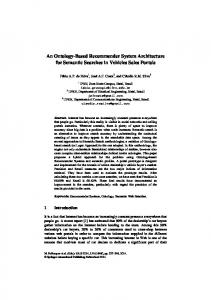
Figure 1: An Illustration Example. The MSR problem involves the recommendation of a sequence of pick-up points and has combinatorial complexity in nature. However, this problem is practically important and interesting, since it helps to improve the business performances of taxi companies, the efficient use of energy, the productivity of taxi drivers, and the user experiences. The MSR problem is different from traditional Traveling Salesman Problem (TSP) [4], which finds a shortest path that visits each given location exactly once. The reason is that TSP evaluates a combination of exact N given locations. In other words, all N locations have to be involved. In contrast, the proposed MSR problem is to find a subset locations of given N locations for recommendation. Also, the MSR problem is different from the traditional scheduling problem [8, 17], which selects a set of duties for vehicle drivers. The reason is that all these duties are determined in advance, such as delivering the packages to determined loca-

2.2

90

45

80

40

70

Lemma 1. Given a set of pick-up points C, where |C| = → ≤ N and Cox(F) = 1, the complexity of searchN , 1 ≤ L− Ri − → ing an optimal directed sequence from R is O(N !) Proof. The complexity of searching an optimal sequence is equal to the total number M of all possible sequences generated from C. Since every directed sequence is actually a permutation of pick-up points which form the subset of C, we decompose the checking process into two steps: enumeration of non-empty subset B from C and the permutation of pick-up points belonging to the subset B. For a subset ¡ ¢ B with i different pick-up points, there are totally Ni different subsets. And the range of integer i is 1 ≤ i ≤ N . For each subset B of i different element, there are totally i! different permutations. Thus the total number ofP all possible directed sequences generated from C is ¡N ¢ M = N · i! < N !(1 + 1 + 1/2) = 52 · N !. Thus, we i=1 i can have 2 · N ! < M < 25 · N !. Therefore, the complexity of search optimal directed sequence is O(N !).

The MSR Problem with Constraints

As illustrated above, it is computationally prohibited to search for the optimal solution of the general MSR problem. Therefore, from a practical perspective, we consider a simplified version of the MSR problem. Specifically, we put a → . In constraint on the length of a recommended route L− Ri other words, the length of a recommended route is set to be → = L. To simplify the discussion, a constant; that is, L− Ri −→ let RiL denote the recommended route with a length of L. Based on this constraint, we can simplify the original objective function of the MSR problem as follows.

Frequency of Occupancy Rates

50

35 30 25 20 15 10

0

60 50 40 30 20 10

5 0

100

(a)

200 300 Driving Hours

400

Driving Hours

500

0

0

0.1

(b)

0.2

0.3 0.4 Occupancy Rate

0.5

0.6

0.7

Occupancy Rates

Figure 2: Some Statistics of the Cab Data. The MSR Problem with a Length Constraint Objective: Recommending an optimal sequence −→ −→ − → L L R (R ∈ R). The goal is to minimize the PTD: −→ min F (P oCab, RiL , P−→ ) L

Analysis of Computational Complexity

Here, we analyze the computational complexity of the MSR problem. A brute-force method for searching the optimal recommended route has to check all possible sequences − → in R. If we assume the cost for computing the function F once is 1 ( Cox(F) = 1), the complexity of searching a given set C with N pick-up points is as follows.

2.3

Frequency of Driving Hours s

tions, while the MSR problem consists of uncertain pick-up jobs among several locations. Figure 1 shows an illustration example. In the figure, for a cab T, the closest pick-up point is C1. However, we cannot simply recommend C1 as the first stop in the recommended sequence even if the probability of having a customer at C1 is greater than C4 which is the second closest to T. The reason is that there is still probability that this cab drive cannot find a customer at C1 and then it will cost much more to go to a next pick-up point. Instead, if T goes to C4 first, T might be able to exploit a sequence of pick-up opportunities. For the MSR problem, there are two major challenges. First, how to find reliable pick-up points from the historical data and how to estimate the successful probability at each pick-up point? Second, there is a computational challenge to search an optimal route.

−→ → − RiL ∈ R

Ri

The computational complexity of this simplified MSR problem is analyzed as follows. → = L and Cox(F ) = 1, the Lemma 2. Given |C| = N ,L− Ri computational complexity of searching an optimal directed − → sequence with a length of L from R is O(N L )

Proof. Since the length of the recommended route has been fixed, the computational complexity can actually be obtained through ¡ ¢ modifying equation in proof of Lemma 1 as M = N · L!, where M is the number of all the L sequences with a length as L. M can be transformed as N (N − 1) · · · (N − L + 1). Thus, the computational complexity of this problem is O(N L ). The above shows that the computational cost of this simplified MSR problem will dramatically increase as the number of pick-up points N increases. In this paper, we focus on studying the MSR problem with a length constraint.

3.

RECOMMENDING POINT GENERATION

In this section, we show how to generate the recommending points and compute the probability of pick-up events at each recommending point from location traces of cab drivers.

3.1

High-Performance Drivers

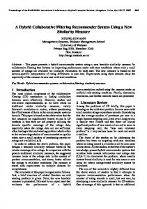
In real world, there are always high-performance experienced cab drivers, who typically have sufficient driving hours and higher customer occupancy rates - the percentage of driving time with customers. For example, Figure 2 (a) and (b) show the distributions of driving hours and occupancy rates of more than 500 drivers in San Francisco over a period of about 30 days. In the figure, we can clearly see that the drivers have different performances in terms of occupancy rates. Based on this observation, we will first extract a group of high-performance drivers with sufficient driving hours and high occupancy rates. The past pick-up records of these selected drivers will be used for the generation of potential pick-up points for recommendation.

3.2

Clustering Based on Driving Distance

After carefully observing historical pick-up points of highperformance drivers, we notice that there are relative more

event happening after going through the suggested route. This probability is P (C1 ) · P (C2 ) · P (C3 ) · P (C4 ). In this paper, since we only consider the driving routes with a fixed length, the travel distance beyond the last pick-up point is set to be D∞ equally for all suggested driving routes. Formally, we represent the distribution of the travel distance before next pick-up event with two vectors: D−→ =hD1 , (D1 + RL =hP1 , D2 ), (D1 +D2 +D3 ), (D1 +D2 +D3 +D4 ), D∞ i and P−→ L

C1 D1

C4 P(C1) D2

D4

P(C4)

PoCab D3 C2

C3 P(C3)

P(C2)

R

Figure 3: A Recommended Driving Route. pick-up events in some places than others. In other words, there are the cluster effect of historical pick-up points. Therefore, we propose to cluster historical pick-up points of highperformance drivers into N clusters. The centroids of these clusters will be used for recommending pick-up points. For this clustering algorithm, we use driving distance rather than Euclidean distance as the distance measure. In this study, we perform clustering based on driving distance during different time periods in order to have recommending pick-up pointers for different time periods. Another benefit of clustering historical pick-up points is to dramatically reduce the computational cost of the MRS problem.

3.3

Probability Calculation

For each recommended pick-up point (the centroid of historical pick-up cluster), the probability of a pick-up event can be computed based on historical pick-up data. The idea is to measure how frequent pick-up events can happen when cabs travel across each pick-up cluster. Specifically, we first obtain the spatial coverage of each cluster. Then, let #T denote the number of cabs which have no customer before passing a cluster. For these #T empty cabs, the number of pick-up events #P is counted in this cluster. Finally, the probability of pick-up event for each cluster (each recommended pick-up point) can be estimated as follows. P (Ci )1≤i≤N =

#P , #T

(2)

where #P and #T are recorded for each historical pick-up cluster at different time periods.

4.

SEQUENTIAL RECOMMENDATION

In this section, we design mobile sequential algorithms for searching the optimal route for recommendation.

4.1

The Potential Travel Distance Function

First, we introduce the Potential Travel Distance (PTD) function, which will be exploited for algorithm design. To simplify the discussion, we illustrate the PTD function via an example. Specifically, Figure 3 shows a recommended driving route P oCab → C1 → C2 → C3 → C4 for the cab P oCab, where the length of suggested driving route L = 4. −→ When a cab driver follows this route RL , he/she may pick up customers at each pick-up point with a probability P (Ci ). For example, a pick-up event may happen at C1 with the probability P (C1 ), or at C2 with the probability P (C1 )P (C2 ), where P (Ci ) = 1 − P (Ci ) is the probability that a pick-up event does not happen at Ci . Therefore, the travel distance before a pick-up event is discretely distributed. In addition, it is possible that there is no pick-up

P (C1 ) · P (C2 ), P (C1 ) · P (C2 ) · P (C3 ), P (C1 ) · P (C2 ) · P (C3 ) · P (C4 ), P (C1 ) · P (C2 ) · P (C3 ) · P (C4 )i. Finally, the Potential Travel Distance (PTD) function F is defined as the mean of this distribution as follows. F = D−→ · P−→ L L R

R

(3)

where · is the dot product of two vectors. From the definition of the PTD function, we know that the evaluation of a suggested drive route is only determined by the probability of each pick-up point and the travel distance along the suggested route, except the common D∞ . These −→ two types of information associated with each drive route RiL can be represented with one 2L-dimensional vector DP = hDP1 , · · · , DPl , · · · DP2L i. Let us consider the example in Figure 3, where L = 4. The 8-dimensional vector DP for this specific driving route is DP = hD1 , P (C1 ), D2 , P (C2 ), D3 , P (C3 ), D4 , P (C4 )i. However, to find the optimal suggested route, if we use a brute-force method, we need to compute the PTD for all directed sequences with a length L. This involves a lot of computation. Indeed, many suggested routes can be removed without computing the PTD function, because all pick-up points along these routes are far away from the target cab. Along this line, we identify a monotone property of the Function F as follows. Lemma 3. The Monotone Property of the PTD Function F . The PTD Function F (DP) is strictly monotonically increasing with each attribute of vector DP, which is a 2Ldimensional vector. Proof. A proof sketch is as follows. By the definition of the function F in Equation 3, we can first derive the polynomial form of F. From the polynomial form of F , we can observe that the degree of each variable is one. Also, D∞ is assumed to be one big enough constant. To prove the monotonicity of F, it is equally to prove that the coefficient of each variable is positive. This is easy to show. The proof details are omitted due to the space limit.

4.2

The LCP Algorithm In this subsection, we introduce the LCP algorithm for finding an optimal driving route. In LCP , we exploit the monotone property of the PTD function and two other pruning strategies, Route Dominance and Constrained Subroute Dominance, for pruning the search space. Definition −→ 1. Route Dominance. A recommended driving route RL , associated with the vector DP, dominates an−→ eL , associated with the vector DP, g iff ∃1 ≤ l ≤ other route R g l and ∀1 ≤ l ≤ 2L, DPl ≤ DP g l . This can be 2L, DPl < DP −→ −→ eL . denoted as RL ° R

By this definition, if a candidate route A is dominated by a candidate route B, A cannot be an optimal route. Next, we provide a definition of constraint sub-route dominance.

The skyline route query retrieves all the skyline routes − → with a length of L. Formally, we use R Skyline to represent the set of all the skyline routes.

Definition 2. Constrained Sub-route Dominance. − → − → Consider that two sub-routes R sub and R0 sub with an equal length (the number of pick-up points) and the same source − → and destination points. If the associated vector of R sub dom− →0 − → inates the associated vector of R sub , then R sub dominates − → − → − → R0 sub , i.e. R sub ° R0 sub .

Lemma 4. Joint Principle of Skyline Routes and the PTD Function F. The optimal driving route determined by the PTD function F should be a skyline route. This −→ − → is denoted as RL ∈ R Skyline

C′3

D′3 C2

P(C′3)

D3

D4

D’4 C4 P(C4)

C3 P(C3) Figure 4: Illustration: the Sub-route Dominance. − → For example, as shown in Figure 4, R sub is C2 → C3 → C4 − →0 and R sub is C2 → C30 → C4 . The associated vectors of − → − → R sub and R0 sub are DP sub = hD3 , P (C3 ), D4 , P (C4 )i and DP 0sub = hD30 , P (C30 ), D40 , P (C4 )i respectively. Then the − → − → dominance of R sub over R0 sub is determined by the dominance of these two vectors. Here, we have the constraints that two routes have the same length as well as the same source and destination. The constrained sub-route dominance enables us to prune the search space in advance. This is shown in the following proposition. Proposition 1. LCP Pruning. For two sub-routes A and B with a length L, which includes only pick-up points, if sub-route A is dominated by sub-route B under Definition 2, the candidate routes with a length L which contain sub-route A will be dominated and can be pruned in advance. − → Let us study the example in Figure 4. If L = 3 and R sub (C2 − →0 → C3 → C4 ) dominates R sub (C2 → C30 → C4 ), the candidate P oCab → C2 → C3 → C4 dominates the candidate P oCab → C2 → C30 → C4 by Definition 1. Thus we can − → prune the candidate contains R0 sub in advance before online recommendation. Specifically, the LCP algorithm will enumerate all the L-length sub-routes, which include only pick-up points, and prune the dominated sub-routes by Definition 2 offline. This pruning process could be done offline before the position of a taxi driver is known. As a result, LCP pruning will save a lot of computational cost since it reduces the search space effectively.

4.3

The SkyRoute Algorithm

In this subsection, we show how to leverage the idea of skyline computing for identifying representative skyline routes among all the candidate routes. Here, we first formally define skyline routes. Definition 3. Skyline Route. A recommended driv−→ −→ − → −→ ing route RL is a skyline route iff ∀RiL ∈ R, RiL cannot −→ −→ −→ dominate RL by Definition 1. This is denoted as RiL 1 RL .

Proof. (Proof Sketch.) This lemma can be proved by −→ contradiction. Assume that RL 1 is an optimal driving route −→ and is not a skyline route. By Definition 3, RL 1 must be −→ L dominated by some driving route denoted as (Ri ), which is a skyline route. By Definition 1, each attribute of the vector −→ associating with RL 1 should be not smaller than the corre−→ sponding attribute of the vector associating with RiL . Also, there must be one attribute, for which the value of vector −→ associating with RL 1 is bigger than that of vector associating −→ with associating with RiL . Then, by Lemma 3, the function −→ F value of the vector associating with RiL should be less −→ −→ L than that of the vector associating with RL 1 . Therefore, R1 should not be the optimal drive route. With the joint principle of skyline routes and the PTD function F in Lemma 4, it is possible to first find skyline routes and then search for the optimal driving route from the set of skyline routes. This way can eliminate lots of candidates without computing the PTD function F. Next, we show how to compute skyline routes. Indeed, skyline computing, which retrieves non-dominated data points, has been extensively studied in the database literature [9, 11, 13, 18]. However, most of these algorithms cannot be directly used to find skyline routes in the MSR problem, because vectors associated with suggested routes are generated through an expensive cluster network traversal process. In Particular, the performances of traditional skyline computing algorithms degrade significantly when the network size increases or the length of suggested driving route is increased. Also, there are a large memory requirement for storing these vectors during the traditional skyline computing process. Moreover, for real-world applications, the position of empty cab is dynamic. Therefore, the recommended driving routes are dynamic in a real-time fashion. This means that we cannot have the indices for the multidimensional data points(vector DP) in advance, which is desired for many traditional skyline computing algorithms [19]. To this end, we design a SkyRoute algorithm for computing skyline routes by exploiting the unique properties of skyline routes for the purpose of efficient computation. The basic idea of the SkyRoute algorithm is to prune some candidate routes, which are comprised of the dominated sub-routes and cannot be skyline routes, at a very early stage. This idea is based on the observation that any recommended driving routes are composed of sub-routes and different routes can cover the same sub-routes. The search space will be significantly reduced, since lots of candidate routes containing the dominated sub-routes will be discarded from further consideration as skyline routes. In the following, we first introduce two propositions for candidate routes pruning based on dominated sub-routes.

Proposition 2. Backward Pruning. If a sub-route R1 from P oCab to an intermediate pick-up point Ci is dominated by another sub-route R2 from P oCab to Ci under the sub-route dominance By Definition 2, then all the candi−→ date routes RL 3R1 , which have R1 as a precedent sub-route −→ will be dominated by the candidate routes RL 3R2 . The only −→ −→ different between RL 3R1 and RL 3R2 is from P oCab to Ci . −→ Therefore, those candidate routes RL 3R1 can be pruned in advance. Proposition 3. Forward Pruning. If a sub-route R1 from one pick-up point Ci to another pick-up point Cj is dominated by another sub-route R2 from Ci to Cj under the sub-route dominance by Definition 2, then all the candidate −→ routes RL 3R1 , which contain R1 as sub-route will be dom−→ inated by the candidate routes RL 3R2 . The only difference −→ − → between RL 3R1 and RL 3R2 is from Ci to Cj , Therefore, −→ those candidate routes RL 3R1 can be pruned in advance. With the proposition of Backward Pruning, it is possible to decide some dominated sub-routes and discard some candidate routes which contain these dominated sub-routes. Also, the benefit of the proposition of Forwarding Pruning is the ability to prune some dominated sub-routes as well as some candidate routes offline, since both probabilities and distances between pick-up points can be obtained before any online recommendation of driving routes. Note that only sub-routes with a length less than L need to be considered in the above discussion. Figure 5 shows the pseudo-code of the SkyRoute algorithm. As can be seen, during offline processing, SkyRoute checks the dominance of sub-routes with a length L by Definition 2 and prunes the ones dominated by others. This process is also applied in the LCP algorithm. In addition, SkyRoute can also prune sub-routes with different lengths with Forward Pruning in proposition 3. During online processing, results of offline processing are used as candidate routes. From line 2 to line 5, SkyRoute iteratively checks the sub-routes with P oCab as the source node and prunes the candidate routes containing dominated sub-routes with Backward Pruning in proposition 2. Then, in line 6, the candidate set is obtained after all the pruning process. Finally, a skyline query [18] is conducted on this candidate set to find skyline routes. Note that the online search time of the optimal driving route should include the time of online process of SkyRoute and the search time on the set of skyline routes.

4.4

Obtaining the Optimal Driving Route

For both LCP and SkyRoute algorithms, after all the pruning process, we will have a set of final candidate routes for a given taxi driver. To obtain the optimal driving route, we can simply compute the PTD function F for all the remaining candidate routes with a length L. Then, the route with the minimal PTD value is the optimal driving route for this given taxi driver.

4.5

The Recommendation Process

Even though we can find the optimal drive route for a given cab with its current position, it is still a challenging problem about how to make the recommendation for

ALGORITHM SkyRoute(C,P,Dist,L,P oCab) Input: C: set of cluster nodes with central positions P: probability set for all cluster nodes Dist: pairwise drive distance matrix of cluster nodes L: the length of suggested drive route P oCab: the position of one empty cab Output: − → R Skyline : list of skyline drive routes. Online Processing 1. Enumerate all candidate routes by connecting P oCab with each sub-route of RL sub obtained in step 10 during Offline Processing 2. for i = 2 : L − 1 3. Decide dominated sub-routes with ith intermediate cluster and prune the corresponding candidates by using proposition 2 4. Update the candidate set by filtering the pruned candidates in step 3 5. end for 6. Select the remained candidate routes with length of L from the loop above − → 7. Final typical skyline query to get R Skyline from those candidate routes in step 6 Offline Processing(LCP ) 8. Enumerate all sub-routes with length of L from C 9. Prune and maintain dominated Constrained Sub-routes with length of L using proposition 3 10. Maintain the remained non-dominated sub-routes with length of L, denoted as RL sub

Figure 5: The SkyRoute Algorithm many cabs in the same area. In this section, we address this problem and introduce a strategy for the recommendation process in the real world. A simple way is to suggest all these empty cabs to follow the same optimal drive route, however there is naturally an overload problem, which will degrade the performance of the recommender system. To this end, we employ load balancing techniques [10] to distribute the empty cabs to follow multiple optimal drive routes. The problem of load balancing has been widely used in distributed systems for the purpose of optimizing a given objective through finding allocations of multiple jobs to different computers. For example, the load balancing mechanism distributes requests among web servers in order to minimize the execution time. For the proposed mobile recommendation system, we can treat multiple empty cabs as jobs and multiple optimal drive routes as computers. Then, we can deal with this overload problem by exploiting existing load balancing algorithms. Specifically, in this study, we apply the circulating mechanism for the recommender systems by exploiting a Round Robin algorithm [22], which is a static load balancing method. Under the circulating mechanism, to make recommendation for multiple empty cabs, a round robin scheduler alternates the recommendation among multiple optimal drive routes in a circular manner. As shown in Figure 6, we could search k optimal drive routes and recommend the NO.1 route to the first coming empty cab. Then, for the second empty cab, the NO. 2 drive route will be recommended. Assume there are more than k empty cabs, recommendations are repeated from NO. 1 route again after the kth empty cab. In practice, to achieve this, one central dispatch (processor) is needed to maintain the empty cabs and as-

NO.2

5.2

NO.3

Multiple Empty Cabs

NO.1

K drive routes

NO.k

NO. NO.ii

NO.k-1

Figure 6: Illustration of the Circulating Mechanism. signments among the top-k driving routes. Note that the load balancing techniques are not the focus of this paper.

5.

An Illustration of Optimal Driving Routes

Here, we show some optimal driving routes determined by the PTD function F on real-world data. In Figure 7, we plot the potential pick-up points within the time period 6P M -7P M and the assumed position of the target cab for recommendation. During this time period, the optimal drive routes evaluated by the PTD function are P oCab → C1 → C3 → C2, P oCab → C1 → C3 → C2 → C7 and P oCab → C4 → C1 → C3 → C2 → C7 for L = 3, L = 4 and L = 5 respectively. Please note that we have documented more results and illustrations in a Web site listed in Appendix.

EXPERIMENTAL RESULTS

C2 C6

In this section, we evaluate the performances of the proposed two algorithms: LCP and SkyRoute.

C3 C4

PoCab

5.1

The Experimental Setup

Real-world Data. In the experiments, we have used real-world cab mobility traces, which are provided by the Exploratorium - the museum of science, art and human perception through the cabspotting project [1]. This data set contains GPS location traces of approximately 500 taxis collected around 30 days in the San Francisco Bay Area. For each recorded point, there are four attributes: latitude, longitude, fare identifier and time stamp. In the experiments, we select the successful cab drivers and generate the cluster information as follows. Specifically, we select cab drivers with total driving hours over 230 and occupancy rates greater than 0.5. In total, we obtain 20 cab drivers and their location traces. Based on this selected data, we generate potential pick-up points and the pick-up probability associated with each pick-up point for different time periods. In the experiments, we focus on two time periods: 2P M 3P M and 6P M -7P M . For these two time periods, we obtain 636 and 400 historical pick-up points respectively. After calculating the pairwise driving distance of pick-up points with the Google Map API, we use Cluto [12] for clustering. All default parameters are used in the clustering process except for ”-clmethod=direct”. Please note that, since the driving distance measured by the Google Map API depends on the driving direction, we use the average to estimate the distance between each pair of pick-up points. Finally, we group the historical pick-up points into 10 clusters. The traveling distances between clusters are measured between centroids of clusters with the Google Map API. Synthetic data. To enhance validation, we also generate synthetic data for the experiments. Specifically, we randomly generate potential pick-up points within a specified area and generate the pick-up probability associated with each pick-up point by a standard uniform distribution. In total, we have 3 synthetic data sets with 10, 15 and 20 pickup points respectively. For this synthetic data, we use the Euclidean distance instead of the driving distance to measure the traveling distance between pick-up points. Also, for both real-world and synthetic data, we randomly generate the positions of the target cab for recommendation. Experimental Environment. The algorithms were implemented in Matlab2008a. All the experiments were conducted on a Windows 7 with Intel Core2 Quad Q8300 and 6.00GB RAM. The search time for the optimal driving route and the skyline computing time are two main performance metrics. All the reported results are the average of 10 runs.

C8

C1 C7

C5 C9

C10

Figure 7: Illustration: Optimal Driving Routes. Table 1: Some Acronyms. BFS: LCP S: SR(BNL)S: SR(D&C)S:

5.3

Brute-Force Search . Search with LCP Search via Skyline Computing algorithm SkyRoute + BN L. Searching via Skyline Computing Algorithm SkyRoute + D&C.

An Overall Comparison

In this subsection, we show an overall comparison of computational performances of several algorithms. First, in SkyRoute, after the pruning process proposed in this paper, we apply some traditional skyline computing methods to find the skylines from the remained candidate set. Here, we employ two skyline computing methods, BN L and D&C [18]. In this experiment, all acronyms of evaluated algorithms are given in Table 1. Note that, for BFS, we only compute the PTD value for all candidate routes one by one and find the maximum value as well as the optimal driving route. Also, most information, such as the locations of potential pick-up points and the pick-up probability, can be known in advance. The online computations are the distance from the target cab to pick-up points and PTD function. Figure 8 shows the online search time of optimal driving routes evaluated by the PTD function for different values of L on both synthetic data and real-world data. The search

time shown here includes all the time for online processing. As can be seen, LCP S outperforms BFS and SR(D&C)S with a significant margin for all different lengths of the optimal drive route on both synthetic and real data. The reason why searching via skyline computing takes longer time than LCP S or BFS is that skyline computing is partially online processing and takes a lot of time. Although we only show the results of the time period 6P M − 7P M , a similar trend has also been observed in other time periods. Due to the space limit, we omit these results here. However, we have documented more results in a Web site listed in Appendix.

3.5

Search Time (Sec)

2.5

0.5

0 10

BFS LCPS SR(D&C)S

60

Search Time (Sec)

Search Time (Sec)

30

6

10

0 3

5

4

5

4

Length of Driving Route(L) (b) Comparisons on Synthetic Data (10 Clusters)

Length of Driving Route(L) (a) Comparisons on Real Data (6−7PM)

Skyline Computing Time (Sec)

20

3

18

20

120

2

0

16

40

3

1

14

Figure 10: A Comparison of Search Time (L = 3) on the Synthetic Data set.

50

4

12

Number of Pick−up Points

6

5

1.5

BNL D&C SkyRoute(BNL) SkyRoute(D&C)

BNL D&C SkyRoute(BNL) SkyRoute(D&C) Skyline Computing Time (Sec)

BFS LCPS SR(D&C)S

2

1

8

7

BFS LCPS SR(D&C)S SR(BNL)S

3

4

80

40 2

Figure 8: A Comparison of Search Time. 1

0 10

0 15

Number of Pick−up Points (a) Comparisons on Synthetic Data (L=3)

LCPS Skyline

LCPS Skyline

0.95

20

3

4

5

Length of Driving Route (L) (b) Comparisons on Real Data (6−7PM)

Pruning Percentage

Pruning Percentage

Figure 11: A Comparison of Skyline Computing 0.85

0.8

points on synthetic data. In the figure, a similar trend of performances can be observed as in Figure 8.

0.75

5.4

0.6

0.65

3

4

5

Length of Driving Route (L) (a) The Pruning Effect on Real Data (6−7PM)

0.4 10

15

20

Number of Pick−up Points (b) The Pruning Effect on Synthetic Data (L=3)

Figure 9: The Pruning Effect In terms of the pruning effect, both LCP and SkyRoute can prune the search space significantly as shown in Figure 9, where we show the pruning ratios of LCP and Skyroute. Note that the pruning ratio is the number of pruned candidates divided by the original number of all the candidates. In addition, for LCP S, the pruning process can be done in advance. This saves a lot of time for online search. In particular, Table 2 shows a comparison of online search time between BFS and LCP S across different numbers of pickup points and different lengths of driving routes on both synthetic and real-world data. As can be seen, LCP S always outperforms BFS with a significant margin. Table 2: A Comparison of Search Time (Second) between BFS and LCP S BFS LCP S BFS LCP S BFS LCP S

10 Synthetic Pick-up Clusters L=3 L=4 L=5 0.051643 0.300211 2.000949 0.043750 0.165401 0.803290 15 Synthetic Pick-up Clusters 0.142254 1.925054 23.517042 0.095364 0.611193 4.322053 Real Data (2-3PM) 0.045933 0.297187 1.991507 0.036736 0.141536 0.622932

Finally, Figure 10 shows the online search time of optimal driving routes (L = 3) across different numbers of pick-up

A Comparison of Skyline Computing

In this subsection, we evaluate the performances of different skyline computing algorithms. This experiment was conducted across different numbers of pick-up points and different lengths of recommended driving routes on both synthetic and real-world data. As shown in Figure 11, SkyRoute with BN L or D&C can lead to better efficiency compared to traditional skyline computing methods. The above indicates that SkyRoute is an effective method for computing Skyline routes. Furthermore, we have observed that the computation cost of BNL or D&C varies on different data sets with the same size of candidate routes. The reason is that BNL or D&C has different computation complexity for the best and worse cases. Therefore, even with the same number of pick-up points and the same length of driving routes, the running time of SkyRoute(BNL), (SkyRoute(D&C) or SR(D&C)S) is different as shown in Figure 11 and Figure 8

5.5

Case: Multiple Evaluation Functions

Here, we show the advantages of searching optimal driving routes through skyline computing. Specifically, we evaluate the following business scenario. When there are business needs for different ways to define optimal driving routes, which can be measured by different evaluation functions. As can be seen in Figure 8 and Figure 10, the search of an optimal driving route via skyline computing does not outperform LCP S or BFS, because it takes the most part of total online processing time for computing skylines. However, for a target cab and fixed potential pick-up points, we only need to compute skylines once. And the search space can be

0.25

BFS LCPS

Search Time with Multiple Evaluation Functions (Sec)

BFS 0.2

SR(D&C)S

[4]

0.15

LCPS

[5]

0.1

SR(D&C)S 0.05

0

Comparisons on Real Data (L=3, 6−7PM)

Comparisons on Synthetic Data (L=3, 10 Clusters)

Figure 12: A Comparison of Search Time for Multiple Optimal Driving Routes pruned drastically as shown in Figure 9. In other words, if the goal is to provide multiple optimal driving routes based on different business needs at the same time. Skyline computing will have an advantage. To illustrate this benefit of skyline computing, we design 5 different evaluation functions (including PTD) to select 5 corresponding optimal drive routes. Note that all these evaluation functions have the monotonicity Property as stated in lemma 3. Due to the space limitation, we omit the details of these evaluation functions. Then, we search five different optimal driving routes simultaneously with the methods shown in Table 1 on both synthetic data and real-world data. Figure 12 shows the comparisons of computational performances with L = 3. As can be seen, SR(D&C)S outperforms LCP S and BFS with a significant margin.

6.

CONCLUDING REMARKS

In this paper, we developed an energy-efficient mobile recommender system by exploiting the energy-efficient driving patterns extracted from the location traces of Taxi drivers. This system has the ability to recommend a sequence of potential pick-up points for a Taxi driver in a way such that the potential travel distance before having customer is minimized. To develop the system, we first formalized a mobile sequential recommendation problem and provided a Potential Travel Distance (PTD) function for evaluating each candidate sequence. Based on the monotone property of the PTD function, we proposed a mobile recommendation algorithm, named LCP . Moreover, we observed that many candidate routes can be dominated by skyline routes, and thus can be pruned by skyline computing. Therefore, we also proposed a SkyRoute algorithm to efficiently compute the skylines for candidate routes. An advantage of searching an optimal drive route through skyline computing is that it can save the overall online processing time when we try to provide different optimal driving routes defined by different business needs. Finally, experimental results showed that the LCP algorithm outperforms the brute-force method and SkyRoute with a significant margin when searching only one optimal driving route. Moreover, the results showed that SkyRoute leads to better performances than brute-force and LCP when there is an online demand for different optimal drive routes defined by different evaluation criteria.

7.

REFERENCES

[1] http://cabspotting.org/. [2] G. Abowd, C. Atkeson, and et al. Cyber-guide: A mobile context-aware tour guide. Wireless Networks, 3(5):421–433, 1997. [3] G. Adomavicius and A. Tuzhilin. Towards the next

[6]

[7]

[8]

[9]

[10]

[11] [12] [13] [14]

[15]

[16]

[17]

[18] [19] [20]

[21]

[22]

generation of recommender systems: A survey of the state-of-the art and possible extensions. TKDE, 2005. D. L. Applegate, R. E. Bixby, and et al. The Traveling Salesman Problem: A Computational Study. Princeton University Press, 2006. O. Averjanova, F. Ricci, and Q. N. Nguyen. Map-based interaction with a conversational mobile recommender system. In The 2nd Int’l Conf on Mobile Ubiquitous Computing, Systems, Services and Technologies, 2008. F. Cena, L. Console, and et al. Integrating heterogeneous adaptation techniques to build a flexible and usable mobile tourist guide. AI Communications, 19(4):369–384, 2006. K. Cheverst, N. Davies, and et al. Developing a context-aware electronic tourist guide: some issues and experiences. In the SIGCHI Conference on Human Factors in Computing Systems, pages 17–24, 2000. M. Dell’Amico, M. Fischetti, and P. Toth. Heuristic algorithms for the multiple depot vehicle scheduling problem. Management Science, 39(1):115–125, 1993. D.Papadias, G. Y.Tao, and B.Seeger. Progressive skyline computation in database systems. ACM TODS, 30(1):43–82, 2005. D. Grosu and A. T. Chronopoulos. Algorithmic mechanism design for load balancing in distributed systems. IEEE TSMC-B, 34(1):77–84, 2004. J.Chomicki, J. P.Godfrey, and D.Liang. Skyline with presorting. In ICDE, pages 717– 719, 2003. G. Karypis. Cluto: http://glaros.dtc.umn.edu/gkhome/views/cluto. T. Kian-Lee, E. Pin-Kwang, and B. C. Ooi. Efficient progressive skyline computation. In VLDB, 2001. B. N. Miller, I. Albert, and et al. Movielens unplugged: Experiences with a recommender system on four mobile devices. In international conference on Intelligent user interfaces, 2003. R. J. Mooney and L. Roy. Content-based book recommendation using learning for text categorization. In Workshop Recom. Sys.: Algo. and Evaluation, 1999. M. Pazzani. A framework for collaborative, content-based, and demographic filtering. Artificial Intelligence Review, 1999. R. Portugal, H. R. Lourenc4o, and J. P. Paixao. Driver scheduling problem modelling. Public Transport, 1(2):103–120, 2009. S.Borzsonyi, K.Stocker, and D.Kossmann. The skyline operator. In ICDE, pages 421–430, 2001. Y. Tian, K. C.K.Lee, and W.-C. Lee. Finding skyline paths in road networks. In GIS, pages 444–447, 2009. A. Tveit. Peer-to-peer based recommendations for mobile commerce. In the 1st international workshop on Mobile commerce, 2001. H. van der Heijden, G. Kotsis, and R. Kronsteiner. Mobile recommendation systems for decision making ’on the go’. In ICMB, 2005. Z. Xu and R. Huang. Performance study of load balancing algorithms in distributed web server systems. In TR, CS213 Univ. of California,Riverside.

APPENDIX

More results have been documented at the Web site: http : //www.pegasus.rutgers.edu/∼yongge/kdd2010/mobile.html