gistic or hyperbolic tangent functions - are approximated by B-spline basis functions and these ... In the proposed solution a special spline approximation of the activation functions will be used. In the rest of ..... algorithms. Nevertheless, a simple example can be considered: if the first derivative of the ac- ..... Manual 4.2, 2000.
1
An efficient hardware implementation of feed-forward neural networks Tam´as Szab´o, G´abor Horv´ath Technical University of Budapest, Department of Measurement and Information Systems, H-1521. Budapest, M˝uegyetem rkp. 9, Bldg. R. I./113. Hungary, E-mail: [szabo, horvath]@mit.bme.hu
������� This paper proposes a new way of digital hardware implementation of nonlinear activation functions in feed-forward neural networks. The basic idea of this new realization is that the nonlinear functions can be implemented using a matrix-vector multiplication. Recently a new approach was proposed for the realization of matrix-vector multipliers which approach can also be applied for implementing nonlinear functions if these functions are approximated by simple basis functions. The paper proposes to use B-spline basis functions to approximate nonlinear sigmoidal functions, it shows that this approximation fulfils the general requirements on the activation functions, presents the details of the proposed hardware implementation, and gives a summary of an extensive study about the effects of B-spline nonlinear function realization on the size and the trainability of feed-forward neural networks.
1 Introduction and motivations Many modeling, control, pattern recognition, etc. tasks can be solved using neural networks. The motivations behind this general applicability are the universal capabilities and adaptive nature of neural networks. Feed-forward neural networks (FFNNs) like multi-layer perceptrons (MLPs) and radial basis function (RBF) networks are universal approximators and classifiers [1], which means that a properly constructed FFNN can approximate any continuous function with arbitrary accuracy or can solve any classification task. On the other hand neural networks are parallel distributed systems and as a consequence rather high speed operation can be achieved if they are implemented in parallel hardware form. A relatively large segment of the possible applications needs this high-speed operation. Real-time recognition of different This work was supported by the Hungarian Fund for Scientific Research (OTKA) under contract T023868
patterns (e.g. recognition of printed or handwritten characters [2], classification of white blood cells [3], fingerprint recognition [4]), etc. certain control tasks, or such measurement problems where complex sensor systems are used [5], etc. require embedded solutions, where relatively small-size, high-speed implementation can be applied only. This paper deals with a new digital hardware implementation, which is based on a recently suggested efficient matrix-vector multiplier architecture [6], [7]. The efficient implementation of a matrix-vector multiplier is based on an the idea, that - if at least one of the multiplicands is constant - the constant multiplicand can be built into the architecture. Using the advantages of the CSD (Canonical Signed Digit) representation and applying bit-level optimization significant hardware complexity reduction can be achieved. Further advantages of this approach are that the resulting architecture performs full-precision computations and allows high-speed pipe-line operation. Feed-forward neural networks implement nonlinear mappings between input and output data:
� � ��� � where
�� and �
(1)
are the weight matrices of the hidden and the output layer, respectively.
Eq. 1 shows, that the critical operations of the neural mapping from the viewpoint of hardware realization are the multiplications required in the calculation of linear combinations, (e.g.
� ) and the elementary nonlinear mappings denoted by ���. The recently proposed multiplier
architecture is a partly parallel partly serial structure. Using this architecture all required multiplications can be calculated in parallel, while every multiplier implements bit-serial operation [6], [7]. This partly parallel partly serial structure is a good compromise between operation speed and hardware complexity. The second critical operation in a feed-forward neural network is the elementary nonlinear mapping that is realized by the activation function in an MLP. The activation functions that must fulfil certain conditions to obtain universal approximator neural networks, are usually implemented by look up tables [8]. This paper proposes a new solution that is also based on the efficient hardware multiplier architecture. In this solution the activation functions - usually logistic or hyperbolic tangent functions - are approximated by B-spline basis functions and these
B-spline based activation functions are realized using the proposed multiplier structure. The application of this multiplier structure for implementing both critical operations, the multiplications and the elementary nonlinear mappings makes it possible to get efficient hardware implementation of MLPs using field programmable gate arrays (FPGAs) or ASICs. FPGA-based neural realizations are ideal solutions for relatively low-cost, medium/high-speed embedded systems, especially if a prototype or a small series of the product is needed. The paper gives a short review of the general requirements of the activation functions, shows that the B-spline based solution fulfil these requirements and details the proposed hardware architecture. The general requirements on an activation function to get the universal approximating capability are rather weak. However, these requirements usually do not deal with the question of the size of the neural network (the number of the hidden neurons) and with the relation between the activation function and the size of the neural network. Moreover, from practical point of view a further important question if a neural network with the required approximating capability can be reached using standard gradient-based error back-propagation training. Whether a selected activation function let the network efficiently trainable or not cannot be determined easily. Also, to determine the optimal size of the network using a selected activation function is a hard task that theoretically has not been solved so far. The paper - in addition to the new way of implementation - gives the results of an extended experimental study for determining the effects of the implemented activation function on the size and the trainability of the network.
2 Requirements against the activation function Several theorems and different approaches exist in the literature, which prove the universal approximation capability of single hidden layer MLP. Good surveys can be found for example in [9] and [10]. These results are different in more points: – They use different conditions and constrains for the activation function and/or they use different error measures. – The proof of a theorem can be constructive or non-constructive. A proof is constructive if it gives an algorithm for computing the appropriate weight set (or it is proved that the weight set is computable on a Turing machine). Unfortunately, even if an algorithm exists it is not sure that the widely used gradient learning algorithms find the solution.
– They do not give practically useful results about the optimal size of the network (at most they can give a - usually too pessimistic - upper limit). Now just the most important theorems are cited from the literature which prove that the presented implementation method is suitable for MLPs and a network with such activation function has the universal approximation capability. Theorem 1 ([11]). Let � ���
�Ê
Ê be any function. Denote � ��� the functions, which can
be realized by the three layered � dimension FFNN with � ��� activation function. Then � ��� is dense in � �Ê � if and only if � ��� is dense in � �Ê � � for every positive integer �.
Here � �Ê � denotes the class of continuous functions over Ê . This theorem is important, because it states, that the results that are achieved for a one-dimensional network can be generalized to higher-dimensional networks. However, the theorem is not constructive. Theorem 2 ([12]). Let � ���
� Ê Ê be a locally bounded piecewise continuous function. Then � ��� is dense in � ���� ��� � for all positive integers � if and only if � ��� is not an algebraic polynomial. Theorem 2 is a comprehensive interpretation of Leshno et al.’s theorem by K˙urkov´a in [10]. It proves the universal approximation capability of the three layered FFNNs under very weak conditions on the activation function. Similar results, or ones with even weaker conditions can be found in [13] using different error norms. It is clear that the key property of the activation function is the non-polynomiality.
3 B-spline based hardware implementation of the activation function 3.1 Implementation technique Our main goal is to find an efficient way for implementing the activation functions. It will be shown in the sequel that an efficient implementation can be obtained if the nonlinear mappings of the activation functions can be expressed as matrix-vector multiplications. In the proposed solution a special spline approximation of the activation functions will be used. In the rest of the paper the approximated activation function will be called spline activation function. A spline function which is a piecewise polynomial function is formed as a linear combination of B-spline basis functions. The univariate B-spline basis functions can be defined in
different ways [14]. A simple definition can be obtained using a recurrence relationship. Denoting the � -th univariate basis function of order � by �� ���, it is defined by:
��
��
��
� � �� � � � � � ��
� � � �� if � � �
�
� �
� ��
� � � �
�� ��
�
��
� ���
�
��
�
� �
�
(2)
(3)
otherwise
where the �� � �
�� ��� form the so called knot sequence which partitions the axis, and ���� � ��� ��� �� is the � -th interval of the partitioned axis.
On each interval the basis function is a polynomial of order � , and at the knots the polynomials are joined smoothly. The basis functions become smoother as the order increases. B-splines are good candidates for implementing the activation functions as: – The B-spline-based construction fully fulfil the requirements detailed in section 2, so an FFNN with spline activation function can approximate any continuous functions with arbitrary accuracy under some very weak conditions. – B-spline is a smooth function, so any function composed of B-splines is also a smooth function. If the order of the spline is � the first �
� � derivatives of the spline exist and under a
certain condition (spline has only knots with multiplicity one) the derivatives are continuous. This makes it possible to use gradient learning rules in the training of the network. – B-splines are basis functions with final support. If the knot (breakpoint) sequence is equidistant all basis functions are similar. This feature is important from the viewpoint of efficient hardware implementation. The properties of the realized sigmoidal function are determined by the knot sequence, the order of the polynomials and the way the spline coefficients are computed. The more segments are used the better approximation can be achieved, however, as it will be shown later efficient hardware implementation can be obtained if not too many segments are used. Next the spline approximation of the activation function will be presented. The basic concept of the proposed activation function implementation method applies equidistant knot sequence. In this case the B-spline basis functions will be similar disregarding their
displacements. The basis functions have finite supports, which means that for a given input a finite number - exactly � - basis functions will be activated, and that for any input value the approximated activation function will be composed of this � basis functions. On the other hand the support of a basis function contains exactly � �� grid points which partitions the basis functions into � segments. This segmentation will be found in the approximated activation function too. This means that the activation function to be approximated will also be partitioned into segments. As all segments of the activation function will be formed as the weighted sum of all basis function segments, first these basis function segments must be calculated, than the weighted sums have to be computed with the predetermined weight values. To compute the basis function segments an alternative expression of the B-splines have to be used. Instead of using the recurrence relationship given in Eq. 3 every segment of a B-spline basis function can be written as a polynomial. The polynomial expressions depend on the order of the B-spline basis function and the knot sequence. For cubic splines (the order of the spline � is 4, which means that 3rd degree polynomials are used) with equidistant knot sequence the
equations are as follows:
� � � �� �� � � � � � � � � �� �� ��� � ��� � � � � � � � � �� ��� ���� �� � � � �
� � � � � � � �� �� ������ � � �
(4)
�
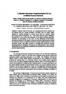
As these segments will be used in the activation function approximation, efficient implementation of the segments is also important. For this implementation a slightly modified version of the previous segments will be used. The modification will shift all segments into the first interval (into the ���
�� interval). These modified segments - which we call standard segments -
are shown in Fig. 1. The modified segments can also be computed as a result of a matrix vector multiplication where a vector of properly chosen powers of the input variable is multiplied by a matrix. The elements of this matrix can be calculated from Eq. 4 if we take into consideration that all segments are shifted into the ���
�� interval.
� � � � � � �� � � � �
�� � � �
�� � � ��
�� �
�� ��� � � �
�� � � ��
� �� � � �
�� � � ��
�� � � �
�� � �
�� � �
�� � �
�� � � � ��� � � � � � � � � � � � � �� ��� �
� � � � ��
(5)
Figure 1. Activated basis functions
Now, as all standard segments are computed, the approximation of the activation function can also be determined. As it was mentioned the activation function will also be partitioned into segments. To determine the value of the approximated activation function for a given input value first the proper segment must be selected then this segment must be evaluated according to the relative position of the input value within this segment. This means that the input values will be separated into two parts: one for the segment selection and the remaining part for determining the relative position within the selected segment. Assuming that � � -bit binary representation form is used, the first several (�� ) MSB bits will be used for segment selection and the remaining bits (��� ) are used as a relative coordinate of the basis function. Certainly, ��
�� � ��� .
1
0.5
0
1
2
3
4
5
6
7
8
−0.5
−1 −1 −0.5 0 0.5 1 Figure 2. Piecewise polynomial activation function; Knots are denoted by circles
In order to work with unsigned digits we will apply a simple displacement transformation:
� �. Thus,
�
� ����� �� �����
� �
� � ��� �
(6)
is the function to be approximated.
��
��� �
���
������ � ��
�
����
Figure 3. Arranging the bits of
To follow the activation function construction let see an example. Let � � ��
and thus
�. This means, that ��� � segments will be used. See Fig. 2. Every segment will be
formed as a weighted sum of the previously implemented B-spline basis function segments. ��
�� �
� �
� � �
� �
� � ��� ��� �
� denotes the weight, and ����� � the support of the corresponding basis function.
(7)
The weights of the basis functions can be selected from a table according to the active interval using as an address. This is a solution of the problem and the block diagram of the necessary hardware is discussed in 3.2. However, we can go a step further and compute all the output values parallel:
� � �� �� � � �
� ���� � � �
�� � � �� � � �
� �� � � �� �
� �
� �� �� �� �� ��
�
��
�
��
��
�
��
��
�
�� .. .
�� .. .
� .. .
�� .. .
���
�
��� ��
�
��� �
�
��� ��
�
��� � � �
�� �
�� ��� � � �
�� ��� � � �
�
� � � � �
� �
(8)
This Eq. 8 and the previous Eq. 5 can be combined as
� � � � ��
��
� � � � � �
� � � �
�� � � �� � �
� ��� � �
� � � � � � � � � �� � � � One can see that both
(9)
� and are constant matrices, thus their product (�
� ) can
be computed in advance. In the final step, the “real” output can be chosen according to . As it was mentioned, a cost-effective matrix-vector multiplier architecture had been developed earlier which can also be used herewith providing an efficient implementation for the non-linear activation function. It is discussed in the next section. 3.2 The hardware The previous section introduced a new implementation idea for activation functions using Bsplines computed in a form of matrix-vector multiplication. The elements of the matrix are constant, while the vector is composed from the different powers of the input. The upper part of the input word is used as an address that selects the active spline piece and puts its value to the output. As one can see, if a � -order B-spline is used the first �
� � powers have to be
computed. Fortunately, these powers must be computed for � which is formed from just the several lower bits of the input signal . After all, two possible block schemes are presented depending on whether
– the whole
� � matrix product is computed, where the result will be a vector and the output
is the properly selected element of this vector (Fig. 4), or – only the necessary vector-vector (inner) product is computed (the fix coefficients are selected). This way directly results in the required activation function value, however in this case non-constant vectors must be multiplied (Fig. 5).
� � � � ��
¾
��� ���� � ��� �� ��
�
����� ������ �
����
��
¿
Figure 4. Implementation using dedicated matrix-vector multiplier
memory address
offset
Coefficient LUT
��
��
� �
�� Figure 5. Implementation using coefficient look-up table
�
The implementation with look-up table requires complex variable-variable multipliers and a memory, which can provide � coefficients in the same time and stores � ��� values. The optimized matrix-vector multiplier depending on the size of the matrix can efficiently replace them. In the implementation a further question may arise: what type of arithmetic should be used in the realization, as so far no bindings were taken on the arithmetics. Either bit-serial, bitparallel or digit-serial arithmetics can be used. The decision depends on the required speed, the accessible amount of hardware and the number of B-spline basis functions. If we have more basis functions, – the B-spline approximation gives more accurate result, – this may allow in some cases to decrease the order of the spline (� ), – which results in simpler hardware, because only lower powers of the input variable have to be computed, – less bits remain for � , that is the computation of its powers is simpler, – more coefficients have to be stored (in the look-up table, or to built into the special matrixvector multiplier) In practice higher order (� � �) splines are rarely applied, because the accuracy of the spline approximation does not increase rapidly for larger orders (see the spline literature, e.g. [14], [15]). Above these qualitative deliberations it is very hard to set up more accurate guidelines. Some empirical experiences should be made in order to choose the good setup respecting the required output accuracy. Table 1. gives the maximum absolute and the mean square error of the spline approximation for different order �
� � � splines and where the number of intervals
are 2,4,8,..., 256.
From these results it can be seen, that fairly good approximation can be reached even using rather few intervals. Selecting the proper structure of approximation one should take into consideration, that the accuracy of approximation depends also on the binary representation of the different segments of the activation function. As in every implementation the accuracy of the activation function depends on the word length applied, so using more segments, obtaining more accurate approximation than the accuracy determined by the word length is needless. The analytical analysis of the effect of finite word length is rather hard, instead extensive simulation
�
� ��� �� 1 2 3 4 5 6 7 8
���� ���� ���� ���� �� �
� � ���� ����
� � � � � � � � �
� ��
MSE
�� � ���� �� � ���� �� � ���� �� � ���� �� ���� �� � ���� �� � �� � �� � ����
� � � � � � � �
�� � ���� �� � �� � �� � ���� �� � ���� �� � ���� �� � ���� �� �� � �� �� ��
� � � � � � � � �
�
� ��
MSE
�� � ��
�� � ���� �� � ���� �� ���� �� � ���
�� � ���� �� ���
�� � ����
� � � � � � � �
�� ��� �� � ���
�� � ���� �� � ���� �� ���� �� �� ���� �� � ��� �� �� ����
� � � � � � � � �
� MSE
�� � ���� �� � ���� �� � ��� �� � ���� �� � ���
�� ���
�� � ���� �� ����
� � � � � � � �
�� � �� �� � �� � �� �� �� � �� �
�� ��
Table 1. The approximation error of the sigmoidal function using different order and different number of intervals of B-splines
�, �
experiments were done. The approximation error is shown in Figure 6. when � and using 8 (�
�
) or 16 (� �) intervals. It can be seen that using 8-bit representation
and 8 intervals the approximation error approximately equals to 2 LSBs (the dotted horizontal lines mark the
�� LSB region), but using 16 intervals this error will be significantly less, than
1 LSB. 0.03
0.03
0.02
0.02
0.01
0.01
0
0
−0.01
−0.01
−0.02
−0.02
−0.03 −1
−0.8
−0.6
−0.4
−0.2
0
0.2
0.4
0.6
0.8
1
a) Figure 6. The approximation error ��
Seeing the �
−0.03 −1
−0.8
−0.6
−0.4
−0.2
0
0.2
0.4
0.6
0.8
1
b)
bit; a) ��� � bit, b) ��� � bit
� case it is obvious, that there is some margin in the allowable error. A
detailed analysis of the elements of
�
shows that this margin can be utilized if the powers
of � are computed with less precision than � . This is caused by the fact that the errors of the
higher order powers of � are in less and less significant in the approximation. So it makes sense to implement the higher order powers with less bits, further reducing the complexity. Figures 7 ... 10 show the errors caused by different precision computations for the case of
�, and the coefficients of �
Figure 6 b) when �
are represented by finite word length.
In the figures �� , � and ��� denote the representation word lengths for the cubic and the
quadratic powers of � and the elements of ��� . In Figure 7 only the coefficients of the basis
function are quantized. In Figures 7 and 9 the powers of � are calculated using 2... 4 bits. The result of both effects is shown in Figure 10. 0.015
0.015
0.01
0.01
0.005
0.005
0
0
−0.005
−0.005
−0.01
−0.01
−0.015 −1
−0.8
−0.6
−0.4
a) �
−0.2
0
, ��
0.2
0.4
0.6
0.8
1
−0.015 −1
0.01
0.01
0.005
0.005
0
0
−0.005
−0.005
−0.01
−0.01
−0.6
a) �
−0.4
−0.2
−0.4
−0.2
0
�
0.015
−0.8
−0.6
, ��� b) � �, � � Figure 7. Error caused by fixed-point arithmetics I
�
0.015
−0.015 −1
−0.8
0
0.2
�, �� �, ���
0.4
0.6
0.8
1
−0.015 −1
−0.8
−0.6
−0.4
−0.2
�
� b) � , �� Figure 8. Error caused by fixed-point arithmetics II
0.2
0.4
0.2
�, ���
0.8
1
0.6
0.8
1
, � ��
�
0
0.6
0.4
�
0.015
0.015
0.01
0.01
0.005
0.005
0
0
−0.005
−0.005
−0.01
−0.01
−0.015 −1
−0.8
−0.6
−0.4
−0.2
0
0.2
0.4
0.6
0.8
1
−0.015 −1
0.01
0.01
0.005
0.005
0
0
−0.005
−0.005
−0.01
−0.01
a) �
−0.2
0
�
0.015
−0.6
−0.4
−0.4
−0.2
0
0.2
0.4
�, �� �, ���
0.6
0.8
1
−0.015 −1
−0.8
−0.6
−0.4
−0.2
0.2
0.4
�, ���
� b) � , �� Figure 9. Error caused by fixed-point arithmetics III
0.015
−0.8
−0.6
�, �� �, ���
a) �
−0.015 −1
−0.8
0
�
b) � , �� Figure 10. Error caused by fixed-point arithmetics IV
0.2
0.6
0.8
1
0.6
0.8
1
�
0.4
�, ���
4 Effect of the application of spline activation functions Theorems presented in section 2 show (necessary and) sufficient conditions for the universal approximation capability of a feed-forward neural network. These theorems do not ensure that a gradient type learning algorithm, like back-propagation - finds the appropriate weight set. Moreover, they are existence theorems, that is they do not provide any point regarding the size of the hidden layer (the number of hidden neurons) to reach a given approximation accuracy. At most, there are upper bounds (or order of magnitude) for the number of hidden neurons,
however, these bounds are too conservative for practical applications. See e.g. [16]. The two most important properties the activation function must have from the viewpoint of gradient learning rules are the existence of the first derivative and the monotony. There is no problem with the derivatives, as B-splines have �
� � derivatives. However, monotony is not automati-
cally guaranteed. According to the knowledge of the authors there is no result in the literature, which proves that monotony of the activation function is necessary for gradient type learning algorithms. Nevertheless, a simple example can be considered: if the first derivative of the activation function changes its sign, the correction term in the learning algorithm goes to wrong direction. We can accept that such disturbances make the error surface more complex with more and more local minima. One knows well, that the convergence of the learning process can stuck at in such local minima, or at least they slow the learning procedure. This is an experimental result, which warns us to beware of using non-monotone activation function. Our implementation method does not tell anything about the derivation of the weights for the spline basis functions. General methods (for interpolating and least-squares splines) can be found in the basic spline literatures ([14], [15]). Unfortunately, these methods do not yield necessarily monotone splines. As this does not influence the implementation method, in this paper we do not pay attention on the computation of monotone spline coefficients, the necessary results can be found in (e.g. [17], [18], [19], [20]). Hereafter simple interpolating splines are used, which may have just tiny non-monotony. The other problem is the optimal number of hidden neurons. In order to clarify the picture the main results of an extensive simulation are presented. for this simulation experiments the teacher-student concept is used [21]. Simulations are done with the following conditions: – Single input, single output teacher net using 5 hyperbolic tangent neurons in the hidden layer is applied. Theorem 1 makes it possible to examine only one dimensional cases and generalize to higher dimensions. However, this theorem does not tell anything about the number of hidden units. Nevertheless, here just the one-dimensional case is discussed, our further task to prove the results for higher dimensional nets. – There were 200 training and 2000 test points selected randomly from a Gaussian distribution. Standard back-propagation training was used with � SNNSv4.2 neurosimulator ([22]).
��� learning rate using the
10−6
10−4
10−7
10−5 MSE
10−3
MSE
10−5
10−8
10−6
10−9
10−7
10−10
4
6
8
10 12 Number of hidden neurons
14
16
10−8
4
6
8
10 12 Number of hidden neurons
14
16
a) Original tangent hyperbolic b) Cubic spline, � pieces Figure 11. Using conventional tangent hyperbolic function a) and cubic B-spline b)
– Activation functions are built up using interpolating splines. The splines approximate the hyperbolic tangent function in the
���� �� interval, the approximated activation function
is constant outside this interval (zero first derivative). The splines have equidistant knot sequences without knot multiplicity using three different number of pieces: 4, 8 and 16. The order of the splines is in the range of �
���. The use of the interpolating spline
approximation results in that the activation function will be slightly non-monotonic close to the saturated region. However, this non-monotonous behavior is small -it is in the range of the LSB. – While all of our spline activation functions approximate the hyperbolic tangent activation ¼ function the derivatives were computed according to � � � � � �� as if the activation
�
function would be the original hyperbolic tangent function. This makes sense, because its computation is very easy and this approximate derivative hides the tiny non-monotonous behavior of the spline activation function. – Number of the hidden neurons is selected as 5,7,9,...15. For each cases we have 10 trial runs.
4.1 Simulation results
Figure 11/a shows the performance of the student network. The lower curve always means the average mean squared error (MSE) in the 200 training points, while the upper curve is for
10−4
10−4
10−5
10−5 MSE
10−3
MSE
10−3
10−6
10−6
10−7
10−7
10−8
4
6
a) �
8
10 12 Number of hidden neurons
14
16
10−8
10−5 MSE
10−5 MSE
10−4
10−6
10−6
10−7
10−7
a) �
10 12 Number of hidden neurons
�
10−4
6
8
b) � order spline, � Figure 12. Using B-spline activation functions I
10−3
4
6
� order spline, � pieces
10−3
10−8
4
8
10 12 Number of hidden neurons
14
16
10−8
4
6
� order spline, � � pieces
8
�
16
14
16
pieces
10 12 Number of hidden neurons
b) � order spline, � Figure 13. Using B-spline activation functions II
14
�� pieces
the 2000 test points. All the MSEs are normalized by the number of points as it is provided by the SNNSv4.2 simulator [22]. 10 runs correspond to a given network size. A fare stage denotes the variance of the 10 runs, the upper and lower ends are for the worst and best errors respectively. The limits of the box are at the 2nd worst and best runs, while the horizontal line in the box is at the middle between the 5th and 6th elements of the ordered errors. A line joints the points in the boxes, which represent the mean values of each 10 runs. We can say that the limit of the precision of the simulation is around � �� �
� � ��
�
�
in term of MSE at training points and
in term of MSE at test points. This performance limit is mainly due to the applied
precision at the representation of the input and desired output point pairs in the simulator or more exactly at the import and export of these points to and from the simulator.
The following experiments can be seen from the simulation results on Fig. 11 . . 13: Concluding remark 1. Nets with B-spline activation functions have poorer performance at the same network size, but increasing the complexity of the network we can decrease the error. This means that more neurons can compensate for the less “nice”activation function. Concluding remark 2. The higher order the B-spline is the better error performance can be obtained at the given network size. Concluding remark 3. The more pieces in the activation function the better error performance can be obtained at the given network size. Concluding remarks 1 and 2 are straightforward. Let we assume a piecewise linear activation function built up from 3 pieces including constant ones. The number of the neurons determines the number of pieces in the approximation provided by the whole net. If there are more neurons this means more pieces for the approximation provided by the whole net. However, this is not so plausible for the remark 3, because if the number of the basis functions is increased in the construction of the B-spline activation function, the number of the independent pieces does not increase regarding the function approximated by the network. This is why the “slope”, the position and the “active region” of a neuron (the influence of its activation function) can be controlled by the weights and we have no more free parameters if just the number of basis functions for the B-spline activation function is increased. Let we see for instance piecewise linear activation functions. The function represented by the network is also piecewise linear one. The input weights of the neuron in the hidden layer determines the distance between two breakpoints at the output of the net which are originally correspond to the breakpoints of the B-spline activation function. Let we choose the th neuron in the hidden layer. Let the input
�� while the output weight value is � . This means that the effect of this neuron at the output of the net is in the interval � ���� � ���� outside it gives a constant � or � . This th neuron provides breakpoints in this � ���� � ���� weight value for this neuron is �� and its bias is
interval equidistantly, that is the linear pieces due to the piecewise polynomial activation function of the th neuron have always the same length and well determined slope. Nevertheless, the shape which has more pieces is closer to a smooth arch and this arch can be controlled by the weights but keeping the pieces of the arch equidistant and correlated. Correlation means here that the ratio of the derivatives of these pieces are fixed (by the B-spline constants).
Conclusion This paper suggests a new and efficient neural network implementation method. A recently suggested efficient matrix-vector multiplier architecture is cited as the basic building block of the NNs. Here it is proved that the nonlinear activation function can also be realized in the form of a matrix-vector multiplication using the B-spline function approximation method. The application of these architectures for both critical operations, the multiplications and the nonlinear mappings results in an efficient dedicated hardware implementation of NNs. Theoretical background of the usage of B-spline activation functions is also discussed and an empirical study was made on the effect of B-spline activation functions to test the performance of the neural networks.
References 1. M.H. Hassoun, Fundamentals of artificial neural networks, MIT Press, 1995. 2. S. Knerr, L. Personnaz and G. Dreyfus, ”Handwritten Digit Recognition by Neural Networks with Single-Layer Training,” IEEE Trans. on Neural Networks, vol. 6, pp. 962–969. 1992. 3. “White blood cell classification & counting with the ZISC,” http://www.fr.ibm.com/france/cdlab/zblcell.htm, 2000. 4. T.G. Clarkson and Y. Ding, RAM-Based Neural Networks, chapter Extracting directional information for the recognition of fingerprints by pRAM networks, pp. 174–185, World Scientific, 1998. 5. J. W. M. Van Dam, B. J. A. Kr¨ose and F. C. A. Groen, ”Adaptive Sensor Models,” Proc. of 1996 International Conference on Multisensor Fusion and Integration for Intelligent Systems, Washington D.C., December 1996, pp. 705–712. 6. Tam´as Szab´o, B´ela Feh´er, and G´abor Horv´ath, “Neural network implementation using distributed arithmetic,” in Proceedings of the International Conference on Knowledge-based Electronic Systems, Adelaide, Australia, 1998, vol. 3, pp. 511–520. 7. Tam´as Szab´o, L˝orinc Antoni, G´abor Horv´ath, and B´ela Feh´er, “An efficient implementation for a matrix-vector multiplier structure,” in Proceedings of IEEE International Joint Conference on Neural Networtks, IJCNN2000, 2000, vol. II, pp. 49–54. 8. Manferd Glesner and Werner P¨ochm¨uller, Neurocomputers, an overview of neural networks in VLSI, Neural Computing. Chapman & Hall, 1994. 9. Franco Scarselli and Ah Chung Tsoi, “Universal approximation using feedforward neural networks: A survey of some existing methods, and some new results,” Neural Networks, vol. 11, no. 1, pp. 15–37, 1998. 10. Vˇera K˙urkov´a, “Approximation of functions by neural networks,” in Proceedings of NC’98, 1998, pp. 29–36. 11. M. B. Stinchcombe and H. White, “Approximating and learning unknown mappings using multilayer networks with bounded weights,” in Proc. of Int. Joint Conference on Neural Networks, IJCNN’90. 1990, vol. III, pp. 7–16, IEEE Press.
12. Moshe Leshno, Vladimir Ya. Lin, Allan Pinkus, and Shimon Schocken, “Multilayer feedforward networks with a nonpolynomial activation function can approximate any function,” Neural Networks, vol. 6, pp. 861–867, 1993. 13. Kurt Hornik, “Some new results on neural network approximatiom,” Neural Networks, vol. 6, pp. 1069–1072, 1993. 14. Carl de Boor, A practical guide to Splines, Springer-Verlag, 1978. 15. Larry L. Schumaker, Spline functions, Basic Theory, Wiley & Sons, 1981. 16. Vˇera K˙urkov´a, “Kolmogorov’s Theorem and Multilayer Neural Networks,” Neural Networks, vol. 5, pp. 501–506, 1992. 17. James T. Lewis, “Computation of best monotone approximations,” Mathematics of Computation, vol. 26, no. 119, pp. 737–747, 1972. 18. Ronald A. De Vore, “Monotone approximation by splines,” SIAM J. Math. Anal., vol. 8, no. 5, pp. 891–905, October 1977. 19. Eli Passow and John A. Roulier, “Monotone and convex spline interpolation,” SIAM J. Numer. Anal, vol. 14, no. 5, pp. 904–909, October 1977. 20. X. M. Yu and S. P. Zhou, “On monotone spline approximation,” SIAM J. Math. Anal., vol. 25, no. 4, pp. 1227–1239, July 1994. 21. D. Saal and S. Solla, “Learning from corrupted examples in multilayer perceptrons,” Tech. Rep., Aston University, UK, 1996. 22. University
of
Stuttgart,
Institute
of
Parallel
and
Distributed
http://www.informatik.uni-stuttgart.de/ipvr/bv/projekte/snns/snns.html, Manual 4.2, 2000.
High-Performance
Systems
(IPVR),
Stuttgart Neural Network Simulator, User