int. j. remote sensing, 2002, vol. 23, no. 18, 3681–3696
An eYcient method for mapping ood extent in a coastal oodplain using Landsat TM and DEM data Y. WANG*, J. D. COLBY and K. A. MULCAHY Department of Geography, East Carolina University, Greenville, NC 27858, USA (Received 11 April 2000; in nal form 9 July 2001) Abstract. An eYcient and economical method for mapping ooding extent in a coastal oodplain is described. This method was based on the re ectance features of water versus non-water targets on a pair of Landsat 7 Thematic Mapper (TM) images ( before and during the ood event), as well as modelling inundation using Digital Elevation Model (DEM) data. Using limited ground observation, most ooded and non- ooded areas derived from this analysis were veri ed. Utilizing only TM data, the total ooded areas in Pitt County, North Carolina on 30 September 1999 was 237.9 km2 or 14.0% of the total county area. This number could be low due to the underestimation of the ooded areas beneath dense vegetation canopies. To further investigate this underestimation, a subset of the area covering the four central topographic quadrangles, the Greenville area, in Pitt County was selected. Through addition of the DEM data into the ood mapping analysis of the Greenville area revealed that the total ooded area was 98.6 km2 (out of a study area of 593.9 km2) or 16.5%. In the Greenville study area, the three landuse and landcover categories most aVected by the ood were bottomland forest/hardwood swamps (32.7 km2), southern yellow pine ( 28.8 km2), and cultivated land (19.1 km2). Their total ooded areas were 80.6 km2 or 81.7% of the total ooded area within this study area. The DEM data helped greatly in identifying the ooding that occurred underneath forest canopies, especially within bottomland forest and hardwood swamps. The method was reliable and could be applied quickly in other coastal oodplain regions using data that are relatively easy to obtain and analyse, and at a reasonable cost. This method should also work well in areas of large spatial extent where topography is relative at.
1. Introduction During an extreme ood event it is important to be able to determine quickly the extent of ooding and the landuse and landcover types under water. This information can be used in developing a comprehensive relief eVort (Corbley 1993). During ooding events remotely sensed data can provide signi cant mapping capabilities. However, obtaining remotely sensed data that represents the ideal combination of ne spatial and temporal sampling, and the ability to see through clouds and/or to discriminate ooding under forest cover is a diYcult task. In addition, accessibility *e-mail:
[email protected] International Journal of Remote Sensing ISSN 0143-1161 print/ISSN 1366-5901 online © 2002 Taylor & Francis Ltd http://www.tandf.co.uk/journals DOI: 10.1080/01431160110114484
3682
Y. Wang et al.
to the data in terms of cost, ease of acquisition, and ease in data processing and analysis are signi cant factors. On 2 September 1999, Hurricane Dennis visited the Outer Banks of North Carolina. It then returned as a tropical storm on 5 September, spreading signi cant precipitation across eastern North Carolina and left the ground saturated. On 15 September 1999, Hurricane Floyd made landfall near the South Carolina–North Carolina border and proceeded to churn through eastern North Carolina, dumping 25–46 cm of rain in many areas in less than 72 h. On 17 September the Tar, Neuse, Roanoke and Pamlico Rivers were predicted to reach ood stage, and to continue to rise for several days. The devastation due to ooding from these storms and two additional precipitation events in late September was immense. Within a few days oodwaters rose and covered over 50 000 km2, causing an unprecedented disaster in the eastern region of state as one of the worst oods in history inundated eastern North Carolina. In addition to the loss of over 50 lives, more than 6000 homes were destroyed and some 44 000 were damaged. Estimates indicated that losses could exceed $6 billion (Gares 1999). In response to the extensive ooding that occurred after Hurricane Floyd in eastern North Carolina, we developed an eYcient method for mapping ood extent that used Landsat 7 Thematic Mapper (TM) imagery, as well as Digital Elevation Model (DEM) data. This method provides ne spatial sampling and determines ooding under forest cover within a oodplain, with data that is relatively inexpensive and easy to obtain, process, and analyse. Studies of mapping ood extent using Landsat TM data (e.g. Dartmouth Flood Observatory 1999) have noted the inability of the imagery to identify ooded areas under forest cover. Jin (1999) developed a ooding index using the Speci c Sensor Microwave/Imager (SSM/I ) data of the Defense Meteorologic Satellite Program (DMSP). Synthetic Aperture Radar (SAR) data can penetrate cloud cover, and have been applied to mapping ooded areas of the Amazon rainforest (e.g. Hess et al. 1995, Melack and Wang 1998, Miranda et al. 1998), monsoon ood damage in Bangladesh (ImhoV et al. 1987), and river ood waves in the Great Upper Mississippi Valley ood of 1993 (Brakenridge et al. 1998). ImhoV et al. (1987) also incorporated the use of Landsat Multi-Spectral Scanner (MSS) data and inventoried landcover classes inundated during ooding. DEMs have been used in various ways to aid in ood mapping and modelling. They have been used as an integral part of a Geographic Information System (GIS) database applied to hydrologic ood modelling eVorts (e.g. Muzik 1996, Correia et al. 1998). They can also be applied towards veri cation of insurance claims after a ood (Barnes 1996). In addition, the delineation of oodplains and the development of ood inundation maps have relied on DEMs (e.g. Jones et al. 1998). The recognition of error in DEMs is an important concern. However, it has been investigated (Brown and Bara 1994), and a few examples have been provided in the literature that is applicable to oodplain mapping (e.g. Lee et al. 1992, Hunter and Goodchild 1995). In this paper, we present a method for mapping ood extent in a coastal oodplain through the use of TM data, as well as DEM data. First, we describe the study area, and the extent of damage due to ooding from the hurricane. Then we provide a discussion of the TM, DEM, and landuse/landcover data and initial processing steps, and describe ground observations. Next, the ood mapping eVorts are explained using TM data for Pitt County, and TM and DEM data for a subset of Pitt County.
Flood mapping using T M and DEM data
3683
We then present the results. We also discuss the potential for applying the ood mapping methods (using TM data alone, and combining TM and DEM data) in coastal oodplains in general, and the limitations and cautions that should be noted when applying these methods to mapping ood extent in areas of large spatial extent, and areas having large topographic variation. 2. Analytical approaches 2.1. Study area and ground observation Most of eastern North Carolina lies within the Atlantic coastal plain. Pitt County lies in the eastern coastal plain of North Carolina, at the approximate centre of the region. The elevation of the area drops only about 60 m as it extends 120–160 km from the Piedmont region in the middle of the state towards the coast. Four large elongated river systems drain the coastal plain in a north-west–south-east direction. Flat broad oodplains are usually located on the northern side of the rivers with higher ground on the south (Gares 1999). In Pitt County the land surface has very low relief and many parts of the region have been extensively drained, cleared and ditched for agricultural use. The soils are primarily characterized as poorly drained or extremely poorly drained (63.0%), with the remaining area consisting of moderately well to well-drained soils (Gares 1999). Pitt County has a population of about 126 000 (estimated in 1998). The largest city, Greenville, is centrally located and has a population of approximately 60 000 (estimated in 1998). The additional residents of the county are spread throughout rural towns. In Pitt County the majority of the 1999 ooding occurred north of the Tar River. The Tar River has been slowly migrating southward towards the drainage divide of the Neuse River so broad primary and secondary oodplains extend northward from the river channel. North and immediately adjacent to the Tar River is a band following the channel that is currently de ned as conservation/open space landuse in the City of Greenville ( gure 1). This conservation/open space landuse zone grades into low and medium density residential, industrial and mixed land uses. It is clear from the photograph, however, that there is signi cant activity within this open space landuse. The City of Greenville alone suVered ooding to its airport, water treatment facility, power transmission substation and numerous residential and industrial areas that are within or nearby current open space landuse zones. In Pitt County, some 6000 homes were ooded. Over three-quarters of these homes were largely uninsured. Upwards of 50 000 people were displaced. More than 6000 were housed in emergency shelters, many for over 3 weeks. Once the oodwaters had completely subsided, but before high water marks faded, ground data information was gathered in the eld. Areas both north and south of the Tar River were examined for the extent and depth of ood waters. The aerial photo ( gure 1) was taken on 23 September 1999 during the ood event and is centred approximately on the City of Greenville. The ood gauge information used for this study was taken from the gauge on the Green Street Bridge ( gure 1). Floodwaters extend into the student housing district seen in the south-eastern section of the photo and throughout the entire area shown north of the river. Areas of extensive tree canopy north of the river in the primary and secondary ood plain were completely ooded. Figure 2 shows the high water marks (reaching the middle of windows) on a house trailer in a trailer park that is located immediately adjacent to the north-eastern most section of the photo. These areas of tree canopy were not
3684
Y. Wang et al.
Figure 1. Aerial photo of a portion of the City of Greenville, North Carolina, taken during the September 1999 ood. The major part of the City of Greenville is on the south side of the Tar River.
classi ed in the TM images as ooded but, clearly, they were ooded to a signi cant depth. 2.2. Remotely sensed data For ood mapping, two sets of the remotely sensed data are required; one set consisting of data acquired before (and as close as possible to) the ood event, and the other acquired during the occurrence of the ood. In reality, data availability may cause some compromise. In this study, the Tar River reached peak ood stage in the area of Pitt County on 21 September 1999. The Landsat 7 TM data that were available closest to this date were acquired on 30 September 1999. Due to the 16-day repeat orbiting of the Landsat 7 satellite, the availability dates for images of pre ood data were 14 September, 29 August, 13 August and 28 July. Due to the severe cloud coverage in the 14 September and August images, we used the image acquired on 28 July for pre- ood analysis. (There were some thin clouds and patches of cloud in the 28 July image that did aVect our analysis.) In summary, we ordered two TM images, one acquired on 28 July 1999, and the other on 30 September 1999. We geo-referenced both images and were able to determine the extent of ooding in Pitt County using the non- ooded 28 July image as a reference. 2.3. DEM data of Greenville area and river gauge readings at Greenville DEM data were available from the United States Geological Survey’s (USGS) web site in the Spatial Data Transfer Standard (SDTS) format. The DEM has a 30 m×30 m resolution, and in this area the elevation interval (z=height) is 0.30 m. The accuracy of the DEM data (i.e. the uncertainty, or root mean square error,
Flood mapping using T M and DEM data
3685
Figure 2. Flooded mobile home in a densely vegetated trailer park on the oodplain, just north of the Tar River, Greenville, North Carolina. The high-water mark reaching the middle of windows is clearly shown on the side of the mobile home.
RMSE) in this area is 1 m. Four 7.5 min USGS topographic quadrangles, Greenville NW, NE, SE and SW were downloaded, imported, and mosaiced. The four mosaiced quads covered an area of about 600 km2. Descriptive statistics for the four-quadrangle DEM area included min.=0 m, mode=11.9 m, median=14.0 m, mean=14.6 m, max.=26.2 m, and standard deviation=6.4 m. This study area is primarily at, especially on the north side of the Tar River where most of the ooding occurred (e.g. gures 1 and 2). We then co-registered the TM and DEM data so that the same area of interest can be easily extracted. Flood stage on the Tar River is measured from a point 0.7 m below sea level (based on the North American Vertical Datum, NAD88). The bottom of the river is about 2 m below sea level. The Tar River leaves its banks 4 m above this measuring point. The Tar River crested at 9.2 m on 21 September. On the date the imagery was taken, 30 September, data from the USGS showed that the mean stage level for the Tar River at the Greenville station was 6.1 m. The non- ood stage surface height of the water in the Tar River according to the river gauge reading on 28 July 1999 was
3686
Y. Wang et al.
1.1 m. Therefore, the elevations that represented ooded areas on 30 September ranged from 1.1 to 6.1 m. These elevations were used as a basis for classifying the area on the Greenville topographic quadrangles into water bodies/rivers, ooded areas, and non- ooded areas, which will be discussed in detail in a later section (see tables 5 and 6). 2.4. North Carolina landuse and landcover data Between 1995 and 1997, the North Carolina Center for Geographic Information and Analysis (NCCGIA), in cooperation with the NC Department of Transportation and United States Environmental Protection Agency Region IV Wetlands Division, contracted Earth Satellite Corporation (EarthSat) of Rockville, Maryland to generate comprehensive landcover data for the entire state of North Carolina (Earth Satellite Corporation 1997). There are 21 landuse and landcover type categories in the entire state data layer. For Pitt County, only 17 categories exist ranging from highly developed areas to unconsolidated sediment areas. To facilitate the presentation of this paper and to provide the reader with a better understanding of the landcover classes, we provide brief de nitions of some categories (in table 3). The three landuse/ landcover categories that were aVected the most by the ood were bottomland forest/ hardwood swamps, southern yellow pine, and cultivated land. Bottomland forests/ hardwood swamps are areas where deciduous, dominant, woody vegetation is above 3 m in height, as well as occurring in lowland and wet areas. Crown density is at least 25%. Southern yellow pine are areas where stocking of trees is 75% evergreen needleleaf or broad-leaf species, including the following forest types: longleaf pine, loblolly-slash pine, other yellow pine, and pond pine. Cultivated lands are areas of land that are occupied by row and root crops that are cultivated in distinguishable rows and patterns. Two other important categories aVected by the oods were high and low intensity developed areas, which contains the housing and infrastructure for the majority of the human population in the area. High intensity developed areas are covered by more than 80% synthetic (man-made) landcover. Low intensity developed areas have between 50 and 80% coverage by synthetic landcover. (See table 3 for the ooded areas for other landuse and landcover types.) 2.5. Flood mapping using T M images The initial goal in ood mapping was to investigate the utility of the TM images for identifying areas that were ooded or not ooded. There were two steps: (1) identify water versus non-water areas on the TM images before and during the ood event, respectively, and (2) compare the areas classi ed as water or non-water on both TM images to determine which areas represented ooding. 2.5.1. Identifying water areas versus non-water areas There are many possible methods for identifying water versus non-water areas using TM data (e.g. Jensen 1996). After unsuccessful trials of using supervised and unsupervised classi cation, and other methods, we used the addition of two TM bands (TM4+TM7) of 28 July, and of 30 September, respectively. TM4 (0.76–0.90 mm, re ective infrared) is responsive to the amount of vegetation biomass, and is useful in identifying land and water boundaries. However, it is possible to confuse water and asphalt areas (road pavements and rooftops of buildings) in the developed areas such as downtown, commercial/industrial areas, etc., as they appear black on the TM4 image or they re ect little back to the sensor. On the TM7
Flood mapping using T M and DEM data
3687
(2.08–2.35 mm, mid-infrared ) image, the re ectance from water, paved road surfaces, and rooftops diVers. Thus, one can identify the water ( ooded ) and non-water (non ooded ) area in the developed areas, by incorporating of TM4 and TM7 into the analysis, as detailed in table 1. This addition is done separately for the July and September TM data. Therefore, the classi cation rule was: If the re ectance of pixels or areas is low in the TM4 plus TM7 image, the pixels represented water, otherwise the pixels represented non-water or dry areas. In the analysis, we noted that the re ectance from water, paved road surfaces, and asphalt rooftops of buildings in the developed areas may be also distinguished on TM5. Thus, TM5 could have been used to detect water versus non-water areas. However, the diVerences on TM5 were slightly smaller than those on TM7 image. Also, Banumann (1996) added two (before and during ood event) TM4 images in his 1993 Mississippi ood analysis. He then sliced the added image into water, ooded areas, and non- ooded areas. He further added TM7 data to the combined TM4 image to separate some confusion between the water and industrial area. Once the representation of the re ectance values for water and non-water features was understood, a cut-oV value could be determined to separate the two categories. For the July TM image, the cut-oV value was 141. If a pixel’s DN value was less than 141, that pixel was assigned as a water category, otherwise it would assigned as a non-water category. For the September TM image, the cut-oV value was 109, i.e. if a pixel’s DN was less than 109, that pixel was classi ed as water, otherwise it was classi ed as non-water. Even though the selection of the cut-oV values may seem to be somewhat arbitrary, we used two diVerent methods to check the cut-oV values. One was ground truthing, and the other was the analysis of the histograms of the TM4 plus TM7 images. In the former, ground observations along the Tar River were used to pick the cut-oV values. These observations were made in the eld in early October of 1999 (e.g. gure 2), and through the analysis of aerial photos taken during the ood event. In the latter, the histogram of the TM4 plus TM7 image was examined to see whether the histogram indicated the cut-oV values. This was the case for the histogram of the July TM4 plus TM7 image; two distinct distributions were observed from the histogram plot. There were also two identi able distributions in the histogram of the September TM4 plus TM7 image. However, a distinct separation between the two distributions, was not as easily identi ed (i.e. any DN value ranging from 107 to 111 may be selected). 2.5.2. Determine ooded areas during the ood event After identifying water versus non-water areas on both images (one acquired before the ood event and the other during the ood ) using the above criteria, determination of areas that were ooded could be made. On a pixel by pixel basis,
Table 1.
Re ectance of water, asphalt pavement (road surface, root of buildings, etc.), and other non-water dry areas on TM4 and TM7 images. Re ectance on TM4 Re ectance on TM7
Water Asphalt pavement Other dry area
low low high
low intermediate high
Re ectance on TM4+TM7 low intermediate high
3688
Y. Wang et al.
there were four possible results, and the following rules were used to determine the ooded areas: 1. If an area was classi ed as water before and during the ood event, it was not considered to be ooded. Water areas in the study areas are the regular river channels, ponds, etc. 2. If an area was classi ed as dry or non-water on the July (pre- ood ) image, and the area was classi ed as water on the September ( ood ) image, the area was considered to be ooded. 3. If an area was dry on both the July and September images, the area was not ooded. 4. It is possible to have an area that was classi ed as water in the July image, classi ed as non-water in the September image. Possible explanations include (a) landuse change between the dates that the imagery was acquired, and (b) cloud eVects on the classi cation. In our analysis, we have noticed the shadows of some small patches of clouds in the July image. The locations shadowed by the cloud were dry in July and September 1999. 3. Results and discussions 3.1. Flood mapping derived by T M images Using the TM data and the method described above, a map representing ooded areas in Pitt County on 30 September 1999, was created ( gure 3). The ooded areas are shown in red and water (regular river channels, ponds, etc.) in blue. The small areas shown as yellow were classi ed as water on the July image, and non-water category on the September image. These areas actually represent the shadows of clouds on the July image. After ground truthing these areas that were non- ooded in September, we recoded this category as non- ooded areas for further analysis (in gure 3). The non- ooded areas are represented by the black/white image of TM band 7 from 30 September. Table 2 summarizes the derived map by the four categories described in §2.5.2. The major ooded areas were along the Tar River owing into Pitt County from the north-west corner of the image and exiting the County to the east. There were large patches of ooded areas in the north. There were ooded areas along the tributary of the Neuse River as well (south-west side of the image, gure 3). 3.2. Areas ooded by each landuse and landcover type Using the landuse and landcover data layer obtained from the NCCGIA, we provide the following description for the derived ood map. The ooded areas along the Tar River and along the tributary of the Neuse River were primarily bottomland forests/hardwood swamps (e.g. gure 1). The patches of ooded areas in the north, north-east, and south-east of the image were mainly southern yellow pines and cultivated lands. The three categories most aVected by the ood, in terms of size and percentage of the total ooded area in Pitt County, were southern yellow pine (91.7 km2 or 5.4% out of the total areas in the County), bottomland forest/hardwood swamps (73.6 km2 or 4.3%), and cultivated lands (40.0 km2 or 2.4%). It should be noted that most of the high and low intensity developed areas were not ooded on 30 September 1999. (The oodwater from the Tar River had receded about 3 m from its crest on 21 September. The main developed areas are near the banks of the Tar River.) It should be also noted that there was a slight diVerence of the sizes of the
Flood mapping using T M and DEM data
3689
Figure 3. The ood extent in Pitt County, North Carolina on 30 September 1999, derived from a pair of Landsat TM images of 28 July and 30 September 1999. The grey rectangle indicates the Greenville study area. Table 2. Flood mapping of Pitt County, North Carolina, as of 30 September 1999. Area ( km2)
Area (%)
Water bodies/Rivers Flooded areas Cloud shadows Non- ooded areas
13.3 237.9 1.2 1444.8
0.8 14.0 0.1 85.1
Total
1697.2
100
water bodies/river channels derived from the TM image pair of 1999 and NCCGIA landuse data layer (13.3 km2 vs 12.2 km2, cf. Tables 2 and 3). This diVerence could be due to diVerent ways to identify water, due to the errors in our analysis and/or
3690
Y. Wang et al.
Table 3. Total areas from the landuse and landcover type data layer and ooded areas of each landuse and landcover type in Pitt County (NC) derived from TM data.
High intensity developed Low intensity developed Cultivated Managed herbaceous cover Unmanaged herbaceous cover—upland Unmanaged herbaceous cover—wetland Evergreen shrubland Deciduous shrubland Mixed shrubland Mixed upland hardwoods Bottomland forest/hardwood swamps Needleaf deciduous Southern yellow pine Mixed hardwoods/conifers Oak/gum/cypress Water bodies/rivers Unconsolidated sediment Total
Total areas from the landuse data layer ( km2)
Flooded areas on 30 Sept. 1999 (km2)
Overall (%)
12.6 22.8 612.8 40.6
1.1 0.9 40.0 3.1
0.1 0.1 2.4 0.2
13.4
0.5
0.0
0.1 177.1 19.5 26.0 0.1
0.0 16.0 1.9 2.3 0.0
0.0 0.9 0.1 0.1 0.0
369.3 0.1 350.5 39.1 0.3 12.2 0.7 1697.2
73.6 0.0 91.7 3.4 0.1 3.1 0.1 237.8
4.3 0.0 5.4 0.2 0.0 0.2 0.0 14.0
in the landuse data layer, due simply to landuse change since the creation of the landuse data layer in 1996, or all three. 3.3. Addition of the DEM data into the ood mapping analysis Due to the dense or continuous canopy coverage in bottomland forest/hardwood swamps and in some dense southern yellow pine stands, and due to the lack of canopy penetration of the TM data, ooded areas under the canopies were not detected by classi cation of the TM data. This underestimation of ooded areas was veri ed through ground truthing and visual interpretation of low-altitude oblique aerial photos taken during the 1999 ood. On the ood map, these undetected ooded areas show up as ‘patches or holes’ along the primary oodplain near the riverbanks. It is important to point out this underestimation, because oods in the coastal oodplains of North Carolina, as well as the entire East Coast and the coast of the Gulf of Mexico often occur from the mid-summer to fall, and trees in the oodplain are almost fully leaf-on during this period of time. Radar data (especially radar data from a long wavelength system) can penetrate the (dense) canopies and identify whether the areas underneath the canopies were ooded or not. However, due to the cost of the radar (such as ERS SAR or Radarsat SAR) data we did not incorporate them in the ood mapping analysis. One alternative is to integrate DEM data into the analysis. There are several advantages to this integration. In the USA, the DEM data are widely available and can be directly download from USGS/EROS web site. (It should be noted that the availability of DEM data in other countries might be limited.) Also, most of the bottomland forest and hardwood swamps in the oodplain are located in places of low elevation or along the banks of rivers. By
Flood mapping using T M and DEM data
3691
using river gauge reading to inundate the DEM, one can map the ood underneath tree canopies in the bottomland forest, and hardwood swamps, as well as in some southern yellow pine stands in low elevation areas. Additionally, high-quality DEM data work well for ood mapping in areas of relatively at terrain, as exists in this study area and other coastal oodplains along the East Coast and the Gulf of Mexico. The following discussion describes the integration of the DEM and TM data for the ood mapping study. We used four 7.5 min quadrangles of USGS DEM data for the Greenville areas. A grey box shown in gure 3 indicates the coverage of the four quads, which includes most of the Tar River in Pitt County. We then extracted the area (of the block, gure 4(a)) from the ood map of Pitt County ( gure 3) derived from the TM data. Black areas on the image represent water bodies/rivers, grey represents ooded areas, and white represents non- ooded areas. A detailed statistical summary of ooded areas for each landuse and landcover type is provided in table 4. The three categories having the largest areas and highest percentage of ooding were southern yellow pine, bottomland forest/hardwood swamps, and cultivated land. We then inundated the DEM based on the river gauge readings before the ood event and on 30 September 1999. The river gauge station is near the centre of the four quads ( gure 1). These readings were 1.1 m preceding the ood event, and 6.1 m on 30 September. Using the rules found in table 5, we reclassi ed the DEM into water bodies/rivers, ooded areas, and non- ooded areas ( gure 4(b)). The simple threshold used for inundating the DEM was possible due to the relatively at terrain (no sinks) away from the river channel within our study area. The ooded areas were located in the oodplain of the Tar River, and ooded areas did not exhibit the canopy ‘holes’ found on the TM images. By inundating the DEM data, ooded areas under the canopies of the bottomland forest and hardwood swamps could be identi ed. At higher elevations and away from the river, the DEM suggested that those areas were dry or there was no ooding. The DEM does not identify water bodies and/or ooded areas at higher elevations. The ooded areas of each landuse and landcover type derived from the DEM data were also tabulated (table 4), and the largest area (22.6 km2) and highest percentage (3.8%) of ooded landcover type was bottomland forest/hardwood swamps. The nal ood map for the Greenville areas was derived by using the logical ‘OR’ operator to combine the ooded areas from either the TM data or the DEM data ( gure 4(c)). Flooded areas located away from the river and at high elevation were identi ed by the TM data. Flooded areas near the river and its tributaries were determined primarily by the DEM and partially by the TM data. No patches or ‘holes’ were visible on the combined ood map. This ‘OR’ logic allows us to extract the best of the TM and DEM data in the ood mapping analysis, and overcame some of the de ciencies of using the TM data or the DEM data alone. The use of both TM and DEM data in ood mapping was straightforward and eYcient. Furthermore, based on our limited ground observation and analysis of aerial photos taken in the study area during the ood, the results were fairly accurate and reliable. 3.4. L imitation of the integration of the DEM data into the ood mapping analysis Although the results derived from the integrated TM and DEM data were very promising, we would like to oVer two cautions regarding the accuracy of the DEM data and inundation of the DEM data using the river stage data. The DEM data, created by USGS, have an estimated accuracy of 1 m (RMSE).
3692
Y. Wang et al.
Figure 4. Integration of the TM and DEM data in the 1999 ood mapping study for areas of four Greenville quadrangles. (a) Extracted ood map (from gure 3) derived from TM data alone, (b) inundated DEM data based on the river gauge reading on 30 September 1999, and (c) nal ood map by combining the TM and DEM data through a logical ‘OR’ for ooded areas.
High intensity developed Low intensity developed Cultivated Managed herbaceous cover Unmanaged herbaceous cover—upland Unmanaged herbaceous cover—wetland Evergreen shrubland Deciduous shrubland Mixed shrubland Mixed upland hardwoods Bottomland forest/hardwood swamps Southern yellow pine Mixed hardwoods/conifers Oak/gum/cypress Water bodies/rivers Unconsolidated sediment Total
0.7 0.3 15.1 2.1 0.0 0.0 7.0 1.1 1.0 0.0 23.2 28.2 1.2 0.0 1.3 0.0 81.2
0.5
0.0 74.3 7.8 9.6 0.1
112.7 123.9 11.4 0.0 4.7 0.1 593.9
Flooded areas derived from TM data ( km2)
9.2 11.9 208.8 18.9
Total areas from the landuse data layer (km2)
3.9 4.8 0.2 0.0 0.2 0.0 13.9
0.0 1.2 0.2 0.2 0.0
0.0
0.1 0.1 2.6 0.4
Overall (%)
22.6 2.0 2.0 0.0 2.0 0.0 42.7
0.0 2.9 0.7 0.4 0.0
0.0
0.2 0.1 8.5 1.3
Flooded areas derived from DEM data ( km2)
3.8 0.3 0.3 0.0 0.3 0.0 7.0
0.0 0.5 0.1 0.1 0.0
0.0
0.0 0.0 1.4 0.2
Overall (%)
32.7 28.8 2.6 0.0 1.3 0.0 98.6
0.0 8.0 1.3 1.1 0.0
0.0
0.8 0.4 19.1 2.5
Flooded areas derived from TM and DEM data ( km2)
5.5 4.9 0.4 0.0 0.2 0.0 16.5
0.0 1.3 0.2 0.2 0.0
0.0
0.1 0.1 3.2 0.4
Overall (%)
Table 4. Total and ooded areas of each landuse and landcover type in Greenville (NC) derived from TM data alone, DEM data alone, and TM and DEM data combined.
Flood mapping using T M and DEM data 3693
Y. Wang et al.
3694
Table 5. Classi cation rules based on the gauge readings before the ood event and on 30 September 1999. (The interval of the DEM data is 0.3 m.) Min. Water bodies/rivers Flooded areas Non- ooded areas
Max. å
>1 >6
å
1 6
In some areas the RMSE may be higher, for example, under canopies due to the DEM generation procedure used by the USGS. We re-ran the analysis with the DEM dataset at ±1 m of the river gauge reading (with the integration of TM data). Recoding the elevation to represent ooding at 1 m less than the river gauge reading did not signi cantly change the pattern of the ood (i.e. 95.3 km2 vs 98.6 km2 total ooded areas and 16.5% vs 16.1%, tables 6 and 4). The elevation data recoded at 1 m above the gauge reading did expand the ood to the north of the river considerably, as this is an area of very low relief (110.4 km2 vs 98.6 km2, tables 6 and 4). Due to the estimated accuracy of the DEM data, the total ooded areas derived from the combination of TM and DEM data in the Greenville areas could vary from 95.3 km2 to 110.4 km2, and the ooded areas from 16.1% to 18.6% of the total study area (table 6). Flooding of the DEM data only works for a reasonable distance from the river gauge from which you measure stage height. This can be a signi cant distance in Table 6. Flooded areas of each landuse and landcover type in Greenville derived from TM and DEM data. The DEM data were set at ±1 m of the river gauge reading of Tar River on 30 September 1999. At 1 m less than the river gauge data
At 1 m above the river gauge data
Flooded Flooded areas ( km2) Overall (%) areas (km2) Overall (%) High intensity developed Low intensity developed Cultivated Managed herbaceous cover Unmanaged herbaceous cover— upland Unmanaged herbaceous cover— wetland Evergreen shrubland Deciduous shrubland Mixed shrubland Mixed upland hardwoods Bottomland forest/hardwood swamps Southern yellow pine Mixed hardwoods/conifers Oak/gum/cypress Water bodies/rivers Unconsolidated sediment Total
0.7 0.3 17.7 2.4
0.1 0.1 3.0 0.4
1.4 1.0 23.6 4.0
0.2 0.2 4.0 0.7
0.0
0.0
0.0
0.0
0.0 7.6 1.3 1.1 0.0
0.0 1.3 0.2 0.2 0.0
0.0 9.3 1.4 1.2 0.0
0.0 1.6 0.2 0.2 0.0
31.8 28.6 2.5 0.0 1.3 0.0 95.3
5.4 4.8 0.4 0.0 0.2 0.0 16.1
35.1 29.3 2.8 0.0 1.3 0.0 110.4
5.9 4.9 0.5 0.0 0.2 0.0 18.6
Flood mapping using T M and DEM data
3695
areas of low relief such as the coastal plain of eastern North Carolina. This is a relatively at region, as shown above by the summary of the statistics of the fourquad DEM data of Greenville. To work in an area of larger spatial extent or large variation of topography (even in a relatively small spatial extent), stage height from other river gauges should be incorporated and an interpolation method developed to adequately represent ood elevation upstream and downstream. This was one reason that we limited the use of the river gauge data collected in Greenville to leave out inundation in the north-west corner and eastern portion of the Tar River in our DEM data ( gure 3). However, in areas where few river gauges exist estimates have to be made. 4. Conclusions A simple and eYcient method for mapping ood extent in a coastal oodplain has been presented. With limited ground observation, most ooded and non- ooded areas derived from the analysis were veri ed. This method was based on a comparison of the re ectance feature of the water versus non-water targets on a pair of TM images (one acquired before and the other during the ood event), as well as by incorporating DEM data into the analysis. The objective of incorporating the DEM data into the analysis was to overcome the limitation of the TM data in distinguishing between ooded areas and forest canopies. Due to the lack of penetration through the vegetation canopies in the forested areas such as in bottomland forest and hardwood swamps, TM data alone could not identify those ooded areas and led to an underestimation of the ooding. This method was reliable and could be used in the other coastal oodplains (such as the East Coast, and the coast of the Gulf of Mexico of the USA), using similar TM images, DEM data, and river stage data. This method should work well for areas of large spatial extent if the (local ) topography is relatively at, as demonstrated in this study. The total ooded areas derived from the TM data alone, on 30 September 1999 for Pitt County, North Carolina were 237.9 km2 or 14.0% of the total county area. This number may be low due to the underestimation of the ooded areas beneath dense vegetation canopies. The landuse/landcover categories most aVected by the ood were the southern yellow pine (91.7 km2), bottomland forest/hardwood swamps (73.6 km2), and cultivated land (40.0 km2). Their total ooded areas were 205.3 km2 or 86.3% of the total ooded areas in the County. Through integrating the classi cation of ooded areas from TM imagery and from inundating a DEM to represent ooding, the following results were obtained for the Greenville area on 30 September 1999. The total ooded area was 98.6 km2 (out of the total study area of 593.9 km2) or 16.5%. The landuse/landcover categories most aVected by ooding were bottomland forest/hardwood swamps (32.7 km2), southern yellow pine (28.8 km2), and cultivated land (19.1 km2). Their total ooded areas were 80.6 km2 or 81.7% of the total ooded area in the studied area. Incorporating the DEM data assisted greatly in identifying the ooding that occurred underneath the forest canopies, especially under the canopies of bottomland forest and hardwood swamps. However, it should be noted that there were two main limitations regarding the integration of DEM data with TM data for ood mapping. One was the use of river gauge readings to inundate the DEM, and the other was the handling of error in the DEM. The authors intend to investigate methods of error representation (e.g. Hunter and Goodchild 1995) in the future. In addition, the US Army Corp of Engineers is currently surveying high-water marks from the
3696
Flood mapping using T M and DEM data
ooding in this area, and this data will be used to assess the accuracy of the DEM in modelling ood extent. Acknowledgements This research was partially funded by a grant to East Carolina University from the Natural Hazards Research and Applications Information Center at the University of Colorado, Boulder, CO, and partially supported by East Carolina University. References Banumann, P. R., 1996, Flood analysis: 1993 Mississippi ood. URL http://umbc7.umbc.edu/ ~tbenja1/baumann/baumann.html, Vol. 4 of Remote Sensing Core Curriculum. Barnes, S. B., 1996, Northwest Flood ‘96: GIS in the face of disaster. Geographic Information Systems, 22–25. Brackenridge, G. R., Tracy, B. T., and Knox, J. C., 1998, Orbital SAR remote sensing of a river ood wave. International Journal of Remote Sensing, 19, 1439–1445. Brown, D. G., and Bara, T. J., 1994, Recognition and reduction of systematic error in elevation and derivative surfaces from 7 -minute DEMs. Photogrammetric Engineering and Remote Sensing, 60, 189–194. Corbley, K., 1993, Remote sensing and GIS provide rapid response for ood relief. Earth Observation Magazine, September, 2, 28–30. Correia, F. N., Rego, F. C., Saraiva, M. D. S, and Ramos, I., 1998, Coupling GIS with hydrologic and hydraulic ood modeling. Water Resources Management, 12, 229–249. Earth Satellite Corporation, 1997, Comprehensive land cover mapping for the state of North Carolina. Final report, March 1997, Rockville, Maryland. Dartmouth Flood Observatory, 1999, DFO-1999-076 ooding from Hurricane Floyd. NASA-supported Dartmouth Observatory. Gares, P., 1999, Climatology and hydrology of Eastern North Carolina and their eVects on creating the ood of the century. North Carolina Geographer, 7, 3–11. Hess, L. L., Melack, J. M., Filoso, S., and Wang, Y., 1995, Realtime mapping of inundation on the Amazon oodplain with the SIR-C/X-SAR synthetic aperture radar. IEEE T ransactions on Geoscience and Remote Sensing, 33, 896–904. Hunter, G. J., and Goodchild, M. F., 1995, Dealing with error in spatial databases: a simple case study. Photogrammetric Engineering and Remote Sensing, 61, 529–537. Imhoff, M. L., Vermillon, C., Story, M. H., Choudhury, A. M., and Gafoor, A., 1987, Monsoon ood boundary delineation and damage assessment using space borne imaging radar and Landsat data. Photogrammetric Engineering and Remote Sensing, 4, 405–413. Jensen, J. R., 1996, Introductory Digital Image Processing: a Remote Sensing Perspective, 2nd edn (Englewood CliVs, New Jersey: Prentice Hall). Jin, Y. -Q., 1999, A ooding index and its regional threshold value for monitoring oods in China from SSM/I data. International Journal of Remote Sensing, 20, 1025–1030. Jones, J. L., Haluska, T. L., Williamson, A. K., and Erwin, M. L., 1998, Updating ood inundation maps eYciently: building on existing hydraulic information and modern elevation data with a GIS. US Geological Survey Open-File Report 98–200. Lee, J., Snyder, P. K., and Fisher, P. F., 1992, Modeling the eVect of data errors on feature extraction from digital elevation models. Photogrammetric Engineering and Remote Sensing, 58, 1461–1467. Melack, J. M., and Wang, Y., 1998, Delineation of ooded area and ooded vegetation in Balbina Reservoir (Amazonas, Brazil) with synthetic aperture radar. Verh Internat Verein L imnol, 26, 2374–2377. Miranda, F. P., Fonseca, L. E. N., and Carr, J. R., 1998, Semivariogram textural classi cation of JERS-1 (Fuyo-1) SAR data obtained over a ooded area of the Amazon rainforest. International Journal of Remote Sensing, 19, 549–556. Muzik, I., 1996. Flood modeling with GIS-derived distributed unit hydrographs. Hydrologic Processes, 10, 1401–1409.