An Efficient Method for Solving Spread Option Pricing Problem ...

Hindawi Publishing Corporation Abstract and Applied Analysis Volume 2016, Article ID 1549492, 11 pages http://dx.doi.org/10.1155/2016/1549492

Research Article An Efficient Method for Solving Spread Option Pricing Problem: Numerical Analysis and Computing R. Company, V. N. Egorova, and L. Jódar Instituto de Matemática Multidisciplinar, Universitat Politécnica de Valéncia, Camino de Vera s/n, 46022 Valencia, Spain Correspondence should be addressed to V. N. Egorova; [email protected] Received 6 September 2016; Accepted 10 November 2016 Academic Editor: Ivan Ivanov Copyright © 2016 R. Company et al. This is an open access article distributed under the Creative Commons Attribution License, which permits unrestricted use, distribution, and reproduction in any medium, provided the original work is properly cited. This paper deals with numerical analysis and computing of spread option pricing problem described by a two-spatial variables partial differential equation. Both European and American cases are treated. Taking advantage of a cross derivative removing technique, an explicit difference scheme is developed retaining the benefits of the one-dimensional finite difference method, preserving positivity, accuracy, and computational time efficiency. Numerical results illustrate the interest of the approach.

1. Introduction Multiasset option pricing problem has two main challenges arising from their high dimensions and the correlations between assets. This is a type of option that derives its value from the difference between the prices of two or more assets. Spread options can be written on all types of financial products including equities, bonds, and currencies. Spread options are frequently traded in the energy market [1]. Two examples are as follows. Crack Spreads. Crack spreads are the options on the spread between refined petroleum products and crude oil. The spread represents the refinement margin made by the oil refinery by “cracking” the crude oil into a refined petroleum product. Spark Spreads. Spark spreads are the options on the spread between electricity and some type of fuel. The spread represents the margin of the power plant, which takes fuel to run its generator to produce electricity. Since the closed form solution is not available for such problems, many numerical methods are employed. Probably the most popular methods of solving multiasset option pricing problems are those around Monte Carlo method and its modifications [2, 3]. However, their simulation are usually time consuming and slow convergent [4].

Analytical-numerical methods are also existing in the literature as it occurs in the one asset case. So, Kirk and Aron [5] provide an approximation method to price a bivariate spread option problem, but it is inaccurate when the strike prices are high [1, 6, 7]. Alexander and Venkatramanan improve Kirk’s approach in [6] based on the hypothesis that the spread option price is the sum of the prices of two compound exchange options which avoids any strike convention. Fourier Transform approach and numerical integration techniques are used by Chiarella and Ziveyi in [8, 9] for numerical evaluation of American options written on two underlying assets. Among the numerical methods we mention the so-called lattice methods [10, 11]. Recently authors in [4] improve the results of [10, 11] and give fast and accurate results although it requires some minor correlation restrictions. Dealing with pure finite difference methods the existence of the cross derivative term in the partial differential equation (PDE) problem due to asset correlation introduces additional challenges in the numerical solution due to the existence of negative coefficient terms in the numerical scheme as well as involving expensive stencil schemes. Both facts may produce numerical drawbacks coming from the dominance of the convection versus the diffusion as well as more expensive computational cost [12–15].

2

Abstract and Applied Analysis

In order to overcome these difficulties the authors have recently proposed several strategies dealing with finite difference approach: high order compact schemes are proposed in [16] using central difference approximations for stochastic volatility Heston model. The authors in [17] use ADI methods and clever discretizations to obtain stable numerical schemes under minor coefficients restrictions in the PDE. The authors of [14, 18] use special finite difference approximations of the cross derivative term based on a seven-point stencil instead of the nine-point stencil scheme resulting from the central finite difference approach. In this paper we continue removing cross derivative approach based on the transformation of the PDE problem initiated in [12] for the case of one asset stochastic volatility Heston model and applied to the Bates stochastic volatility jump diffusion model in [19]. Apart from avoiding negative coefficients in the proposed scheme, it has the additional computational advantage that uses only a five-point stencil. Here we consider spread option pricing problems for both European and American cases. The paper is organized as follows. The first part of the paper deals with European spread call option with payoff 𝑔(𝑆1 , 𝑆2 ) = (𝑆1 − 𝑆2 − 𝐸)+ , depending on two assets 𝑆1 and 𝑆2 and strike price 𝐸 ≥ 0. In Section 2 the PDE with the boundary conditions is established for the spread option pricing problem. In Section 3 we remove the cross derivative term of the PDE using the canonical form transformation method [20]. In that section we also develop the discretization of the continuous European spread call option problem achieving an explicit finite difference scheme. Section 4 is devoted to the study of the properties of the method like consistence and conditional stability and positivity. In Section 5 we extend the study of previous sections to the European spread put option summarizing the main results including the treatment of the boundary conditions. Section 6 deals with American spread option pricing problem using the LCP technique based on the proposed difference scheme. Finally, in Section 7 we illustrate the numerical results computing, simulating, and comparing accuracy and CPU time with other well acknowledge methods. Throughout the paper, we use the following notation: ‖𝐴‖∞ = max {|𝑎𝑖𝑗 | : 1 ≤ 𝑖 ≤ 𝑁, 1 ≤ 𝑗 ≤ 𝑀} will denote a supremum norm for a given matrix 𝐴 = (𝑎𝑖𝑗 ) ∈ R𝑁×𝑀.

2. Spread Option Pricing Problem and Boundary Conditions The price 𝑈(𝑆1 , 𝑆2 , 𝜏) of a spread option is the solution of the PDE 𝜕𝑈 1 2 2 𝜕2 𝑈 1 2 2 𝜕2 𝑈 𝜕2 𝑈 = 𝜎1 𝑆1 2 + 𝜎2 𝑆2 2 + 𝜌𝜎1 𝜎2 𝑆1 𝑆2 𝜕𝜏 2 𝜕𝑆1 𝜕𝑆2 𝜕𝑆1 2 𝜕𝑆2 + (𝑟 − 𝑞1 ) 𝑆1

𝜕𝑈 𝜕𝑈 + (𝑟 − 𝑞2 ) 𝑆2 − 𝑟𝑈, 𝜕𝑆1 𝜕𝑆2

(1)

0 < 𝑆1 < ∞, 0 < 𝑆2 < ∞, 0 < 𝜏 ≤ 𝑇, where 𝜏 = 𝑇 − 𝑡 is the time to maturity 𝑇, 𝑟 is the interest rate, 𝜎𝑖 is the volatility of the asset 𝑆𝑖 , 𝑞𝑖 is the dividend yield of

asset 𝑆𝑖 , and 𝜌 is the correlation parameter; see [1]. Since we consider backwards time, it changes the signs of the coefficients of (1) and instead of a terminal condition the following initial condition is considered: 𝑈 (𝑆1 , 𝑆2 , 0) = 𝑔 (𝑆1 , 𝑆2 ) = max (𝑆1 − 𝑆2 − 𝐸, 0) +

= (𝑆1 − 𝑆2 − 𝐸) .

(2)

The case 𝐸 = 0 corresponds to exchange options that can be reduced to 1D problem by the change of variables 𝑥1 = 𝑆1 /𝑆2 , 𝑐(𝑥1 , 𝜏) = 𝑈(𝑆1 , 𝑆2 , 𝜏)/𝑆2 . Since the numerical solution of European multiasset options requires the selection of a bounded numerical domain and the translation of the boundary conditions to the boundary of the domain, it is important to pay attention to such conditions. For the initial problem (1)-(2) suitable boundary conditions areas follows. (1) For 𝑆1 = 0 the payoff (𝑆1 −𝑆2 −𝐸)+ suggests Dirichlet’s condition 𝑈 (0, 𝑆2 , 𝜏) = 0,

0 < 𝑆2 < ∞, 0 < 𝜏 ≤ 𝑇,

(3)

as one-dimensional call option. (2) Taking the ideas developed by some authors, for instance, Duffy for the case of basket option (see [21], p. 270), for 𝑆2 = 0 we take the value of the closed form solution of the basic Black-Scholes equation of a call for 𝑆1 with given strike 𝐸, 𝑈 (𝑆1 , 0, 𝜏) = 𝑒−𝑟𝜏 (𝐹𝑁 (𝜙1 ) − 𝐸𝑁 (𝜙2 )) ,

(4)

where 𝐹 = 𝑆1 𝑒(𝑟−𝑞1 )𝜏 , 𝜙1 =

𝐹 1 1 [log + 𝜎12 𝜏] , 𝐸 2 𝜎1 √𝜏

(5)

𝜙2 = 𝜙1 − 𝜎1 √𝜏, where 𝑁(𝑥) is the standard normal cumulative distribution function. (3) As 𝑆1 is large versus 𝑆2 + 𝐸, then the behaviour of the solution looks like the asymptotic value of a onedimensional vanilla call option with the strike (𝑆2 +𝐸) for 𝑆1 ≫ 𝑆2 + 𝐸 (see [22], p. 157), 𝑈 (𝑆1 , 𝑆2 , 𝜏) ≈ 𝑒−𝑞1 𝜏 𝑆1 − 𝑒−𝑟𝜏 (𝑆2 + 𝐸) , 𝑆1 ≫ 𝑆2 + 𝐸. (6) (4) For large values of 𝑆2 we assume that the values are almost constants when 𝑆2 changes; therefore we can use Neuman’s boundary condition: 𝜕𝑈 = 0. 𝜕𝑆2

(7)

These boundary conditions will be validated with the numerical examples.


3

3. Removing the Correlation Term and Problem Discretization

From (14) and (15) it follows the expression of the new variables

We begin this section by transforming the PDE problem (1) in order to remove the cross derivative term. Firstly we eliminate the reaction term 𝑟𝑈 by means of the substitution 𝑉 = 𝑒𝑟𝜏 𝑈,

𝑥=

𝜌 1 log 𝑆1 − log 𝑆2 . 𝑦= 𝜎1 𝜎2

(8)

obtaining

̃ 𝜌 log 𝑆1 ; 𝜎1

(16)

Note that

𝜕𝑉 1 2 2 𝜕2 𝑉 1 2 2 𝜕2 𝑉 𝜕2 𝑉 = 𝜎1 𝑆1 2 + 𝜎2 𝑆2 2 + 𝜌𝜎1 𝜎2 𝑆1 𝑆2 𝜕𝑡 2 𝜕𝑆1 𝜕𝑆2 𝜕𝑆1 2 𝜕𝑆2 + (𝑟 − 𝑞1 ) 𝑆1

𝜕𝑉 𝜕𝑉 + (𝑟 − 𝑞2 ) 𝑆2 . 𝜕𝑆1 𝜕𝑆2

𝑦 − 𝑚𝑥 = − (9)

(10)

where

𝑊 (𝑥, 𝑦, 𝜏) = 𝑉 (𝑆1 , 𝑆2 , 𝜏) ,

(11)

1 𝑎22 = 𝜎22 𝑆22 . 2 Therefore, right-hand side of (9) becomes of elliptic type and a convenient substitution to obtain the canonical form is given by solving the ordinary differential equation

(9) takes the following form without cross derivative term 𝜎12 𝜕𝑊 ̃ ̃ 2 𝜕2 𝑊 𝜕2 𝑊 𝜌 𝜕𝑊 𝜌 ) + (𝑟 − 𝑞 − = ( 2 + ) 1 𝜕𝜏 2 𝜕𝑥 𝜕𝑦2 𝜎1 2 𝜕𝑥 +(

𝜎2 𝜎2 𝜌 1 𝜕𝑊 (𝑟 − 𝑞1 − 1 ) − (𝑟 − 𝑞2 − 2 )) , 𝜎1 2 𝜎2 2 𝜕𝑦

̃ 𝜌 log 𝑎1 , 𝜎1

𝑐2 =

log 𝑎2 , 𝜎2

𝑑1 =

̃ 𝜌 log 𝑏1 , 𝜎1

𝜌) are the conjugate roots of 𝑎11 𝑥2 + and (𝜎2 𝑆2 /𝜎1 𝑆1 )(−𝜌 ± 𝑖̃ 𝑎12 𝑥 + 𝑎22 = 0. Solving (12) one gets

𝑑2 =

log 𝑏2 . 𝜎2

−𝜌 ± 𝑖̃ 𝜌 1 log 𝑆2 + log 𝑆1 = 𝐶0 , 𝜎2 𝜎1

By (17) the rhomboid domain has the sides:

(12)

where ̃ = √ 1 − 𝜌2 , 𝜌

(13)

(14)

where one can relate the integration constant 𝐶0 to the new variables by 𝑥 = Im (𝐶0 ) , 𝑦 = −Re (𝐶0 ) .

(19)

In accordance with [23, 24] and (6) we choose the rectangular domain (𝑆1 , 𝑆2 ) ∈ [𝑎1 , 𝑏1 ] × [𝑎2 , 𝑏2 ] = Ω, where 𝑎𝑖 > 0, 𝑖 = 1, 2, are small positive values; 𝑏2 about 3𝐸 and 𝑏1 about 3(𝑏2 + 𝐸). For the transformed problem (19) due to (16), the rectangular domain Ω becomes a rhomboid with vertices 𝐴𝐵𝐶𝐷 (see Figure 1). From (16) let us denote 𝑐1 =

𝑑𝑆2 𝜎2 𝑆2 + (−𝜌 ± 𝑖̃ 𝜌) = 0, 𝑑𝑆1 𝜎1 𝑆1

(18)

(𝑥, 𝑦) ∈ R2 , 0 < 𝜏 ≤ 𝑇.

1 𝑎11 = 𝜎12 𝑆12 ; 2 𝑎12 = 𝜌𝜎1 𝜎2 𝑆1 𝑆2 ;

(17)

By denoting

In order to remove the cross derivative term, note that the right-hand side of (9) is a linear differential operator of two variables and classical techniques to obtain the canonical form of second-order linear PDEs can be applied; see, for instance, chapter 3 of [20]. Under the assumption of correlated variables with −1 < 𝜌 < 1 the sign of the discriminant is 2 − 4𝑎11 𝑎22 = 𝜎12 𝜎22 𝑆12 𝑆22 (𝜌2 − 1) < 0, 𝑎12

𝜌 1 log 𝑆2 , 𝑚 = . ̃ 𝜌 𝜎2

(15)

(20)

𝐴𝐷 = {(𝑥, 𝑦) : 𝑥 = 𝑐1 , 𝑚𝑐1 − 𝑑2 ≤ 𝑦 ≤ 𝑚𝑐1 − 𝑐2 } , 𝐴𝐵 = {(𝑥, 𝑦) : 𝑐1 ≤ 𝑥 ≤ 𝑑1 , 𝑦 = 𝑚𝑥 − 𝑑2 } , 𝐵𝐶 = {(𝑥, 𝑦) : 𝑥 = 𝑑1 , 𝑚𝑑1 − 𝑑2 ≤ 𝑦 ≤ 𝑚𝑑1 − 𝑐2 } , 𝐷𝐶 = {(𝑥, 𝑦) : 𝑐1 ≤ 𝑥 ≤ 𝑑1 , 𝑦 = 𝑚𝑥 − 𝑐2 } .

(21)

4

Abstract and Applied Analysis y

where

A

𝛼1,2 =

D

𝜎12 𝑘 ̃2 𝑘 ̃ 𝜌 𝜌 (𝑟 ) , ∓ − − 𝑞 1 2 ℎ2 𝜎1 2 2ℎ

̃2 𝛼3 = 1 − 𝜌 x

𝑘 1 (1 + 2 ) , ℎ2 𝑚

(25) (26)

𝛼4,5 =

̃2 𝑘 𝜌 2𝑚2 ℎ2 ∓[

(27)

̃ (𝑟 − 𝑞1 − 𝜌

𝜎12 /2)

𝜎1

−

𝑟 − 𝑞2 − 𝜎22 /2 𝑘 ] . 𝜎2 2 |𝑚| ℎ

The discretization of the spatial boundary is given by B

C

𝑃 (𝐴𝐷) = {(𝑥0 , 𝑦𝑗 ) : 0 ≤ 𝑗 ≤ 𝑁𝑦 } ,

Figure 1: Transformed numerical domain.

𝑃 (𝐴𝐵) = {(𝑥𝑖 , 𝑦𝑖 ) : 0 ≤ 𝑖 ≤ 𝑁𝑥 } , The mesh points in the rhomboid domain are (𝑥𝑖 , 𝑦𝑗 ) such that

𝑃 (𝐵𝐶) = {(𝑥𝑁𝑥 , 𝑦𝑗 ) : 𝑁𝑥 ≤ 𝑗 ≤ 𝑁𝑥 + 𝑁𝑦 } ,

𝑥𝑖 = 𝑐1 + 𝑖ℎ, 𝑥𝑖 ∈ [𝑐1 , 𝑑1 ] , 0 ≤ 𝑖 ≤ 𝑁𝑥 , Δ𝑥 = ℎ =

𝑁𝑦 =

𝑃 (𝐷𝐶) = {(𝑥𝑖 , 𝑦𝑁𝑦 +𝑖 ) : 0 ≤ 𝑖 ≤ 𝑁𝑥 } .

𝑑1 − 𝑐1 , 𝑁𝑥

Δ 𝑦 = |𝑚| ℎ,

(22)

𝑑2 − 𝑐2 , |𝑚| ℎ

𝑛 𝑛 𝜕𝑊 𝑤𝑖+1,𝑗 − 𝑤𝑖−1,𝑗 ∼ , 𝜕𝑥 2ℎ

𝑛 𝑤0,𝑗 = 0,

0 ≤ 𝑗 ≤ 𝑁𝑦 , 1 ≤ 𝑛 ≤ 𝑁𝜏 .

(29)

(30)

For 𝐷C with small value of 𝑆2 , we have transformed Black-Scholes solution, so 𝑛 𝑛 𝑛 𝑤𝑖,𝑁 = 𝐹𝑖𝑛 𝑁 (𝜙1,𝑖 ) − 𝐸𝑁 (𝜙2,𝑖 ), 𝑦 +𝑖

𝑛 𝑛 𝜕𝑊 𝑤𝑖,𝑗+1 − 𝑤𝑖,𝑗−1 ∼ , 𝜕𝑦 2 |𝑚| ℎ

0 < 𝑖 < 𝑁𝑥 , 1 ≤ 𝑛 ≤ 𝑁𝜏 ,

(31)

where (23)

𝑛 𝑛 𝑛 𝜕2 𝑊 𝑤𝑖,𝑗+1 − 2𝑤𝑖,𝑗 + 𝑤𝑖,𝑗−1 ∼ , 𝜕𝑦2 𝑚2 ℎ2

𝐹𝑖𝑛 = exp ( 𝑛 = 𝜙1,𝑖

𝑛+1 𝑛 𝜕𝑊 𝑤𝑖,𝑗 − 𝑤𝑖,𝑗 ∼ , 𝜕𝜏 𝑘 𝑛 where 𝑤𝑖,𝑗 ∼ 𝑊(𝑥𝑖 , 𝑦𝑗 , 𝜏𝑛 ), 𝜏𝑛 = 𝑛𝑘. Substituting these finite difference approximations of the derivatives into (19) is approximated by the explicit difference scheme with five-point stencil

𝑛 + 𝛼5 𝑤𝑖,𝑗+1 ,

+

0 𝑤𝑖,𝑗 = (𝑒𝜎1 𝑥𝑖 /̃𝜌 − 𝑒−𝜎2 (𝑦𝑗 −𝑚𝑥𝑖 ) − 𝐸) ,

Boundary condition for side 𝐴𝐷 is as follows:

The approximations of the derivatives appearing in (19) at the point (𝑥𝑖 , 𝑦𝑗 , 𝜏𝑛 ) are as follows:

𝑛+1 𝑛 𝑛 𝑛 𝑛 𝑤𝑖,𝑗 = 𝛼1 𝑤𝑖−1,𝑗 + 𝛼2 𝑤𝑖+1,𝑗 + 𝛼3 𝑤𝑖,𝑗 + 𝛼4 𝑤𝑖,𝑗−1

Both initial and boundary conditions (2), (3), (4), (6), and (7) are transformed throughout (8), (16), (18). For the initial condition we have

0 ≤ 𝑖 ≤ 𝑁𝑥 , 𝑖 ≤ 𝑗 ≤ 𝑖 + 𝑁𝑦 .

𝑦𝑗 = 𝑚𝑥𝑖 − 𝑑2 + (𝑗 − 𝑖) |𝑚| ℎ, 𝑖 ≤ 𝑗 ≤ 𝑁𝑦 + 𝑖.

𝑛 𝑛 𝑛 𝜕2 𝑊 𝑤𝑖+1,𝑗 − 2𝑤𝑖,𝑗 + 𝑤𝑖−1,𝑗 ∼ , 𝜕𝑥2 ℎ2

(28)

(24)

𝜎1 𝑥 + (𝑟 − 𝑞1 ) 𝜏𝑛 ) , ̃ 𝑖 𝜌

𝐹 1 1 [log 𝑖 + 𝜎12 𝜏𝑛 ] , 𝐸 2 𝜎1 √𝜏𝑛

(32)

𝑛 𝑛 𝜙2,𝑖 = 𝜙1,𝑖 − 𝜎1 √𝜏𝑛 .

Side 𝐵𝐶 corresponds to large values of 𝑆1 , so behaviour of the option there leads to 𝑛 = exp ( 𝑤𝑁 𝑥 ,𝑗

𝜎1 𝑥 + (𝑟 − 𝑞1 ) 𝜏𝑛 ) ̃ 𝑁𝑥 𝜌

− (exp (𝜎2 (𝑚𝑥𝑁𝑥 − 𝑦𝑗 )) + 𝐸) , 𝑁𝑥 + 1 ≤ 𝑗 ≤ 𝑁𝑥 + 𝑁𝑦 , 1 ≤ 𝑛 ≤ 𝑁𝜏 .

(33)


5

Boundary 𝐴𝐵 corresponds with the boundary for large values of 𝑆2 . Condition (7) means that component 𝑆2 is constant and the null first derivative is approximated by the 𝑛 𝑛 − 𝑤𝑖,𝑖 )/|𝑚|ℎ = 0, forward difference (𝑤𝑖,𝑖+1 𝑛 𝑛 𝑤𝑖,𝑖 = 𝑤𝑖,𝑖+1 , 1 ≤ 𝑖 ≤ 𝑁𝑥 , 1 ≤ 𝑛 ≤ 𝑁𝜏 .

(34)

4. Positivity, Stability, and Consistency In this section we show that the proposed numerical scheme (24)–(27) presents suitable qualitative and computational properties, such as consistency and conditional positivity and stability. In order to guarantee positivity of the numerical solution let us check the positivity of the coefficients 𝛼𝑖 . From (25) and (27) it is easy to check that coefficients 𝛼1 , 𝛼2 , 𝛼4 , and 𝛼5 of the scheme (24) are positive under the condition ̃ 𝜎1 𝜌 ℎ < min { 󵄨󵄨 󵄨; 󵄨󵄨𝑟 − 𝑞1 − 𝜎12 /2󵄨󵄨󵄨 ̃2 𝜌 󵄨󵄨 󵄨} . 𝜌 (𝑟 − 𝑞1 − 𝜎12 /2) /𝜎1 − (𝑟 − 𝑞2 − 𝜎22 /2) /𝜎2 ]󵄨󵄨󵄨 󵄨󵄨𝑚 [̃

(35)

Coefficient 𝛼3 is positive, if 𝑚2 ℎ2 . 𝑘< 2 ̃ (𝑚2 + 1) 𝜌

(36)

Under conditions (35) and (36), values in interior points 𝑛+1 , 1 ≤ 𝑖 ≤ 𝑁𝑥 − 1; 𝑖 + 1 ≤ of the numerical domain 𝑤𝑖,𝑗 𝑗 ≤ 𝑁𝑦 + 𝑖 − 1, calculated by the scheme (24), preserve nonnegativity from the previous time level 𝑛 at all interior and 𝑛 ≥ 0, 0 ≤ 𝑖 ≤ 𝑁𝑥 ; 𝑖 ≤ 𝑗 ≤ 𝑁𝑦 + 𝑖. boundary points 𝑤𝑖,𝑗 Let us pay attention now to the positivity of the numerical solution at the boundary of the numerical domain. On the boundary 𝐴𝐷 from (30) we have zero values. On the boundary 𝐷𝐶 formula (31) is used preserving the positivity since it is the transformed Black-Scholes formula throughout expression (16). Along the line 𝐴𝐵 we use Neumann boundary condition (34). Therefore, the positivity at the neighbour interior point guarantees the positivity at the boundary. Finally, on the line 𝐵𝐶 boundary conditions are determined by formula (33). This is transformed expression for the asymptotic behaviour of the call option (6) that is positive under the condition 𝑆1max > (𝑆2max + 𝐸) exp ((𝑞1 − 𝑟) 𝜏𝑛 ) , 1 ≤ 𝑛 ≤ 𝑁𝜏 .

(37)

Following the ideas of Kangro and Nicolaides [24], the computational domain has to be large enough to translate the boundary conditions; therefore 𝑆1max ≥ max {(𝑆2max + 𝐸) exp ((𝑞1 − 𝑟) 𝑇) , 3 (𝑆2max + 𝐸)} .

(38)

Therefore, choosing 𝑆1max according to (38) for the trans𝑛 formed problem 𝑤𝑁 ≥ 0 for any 𝑁𝑥 + 1 ≤ 𝑗 ≤ 𝑁𝑥 + 𝑁𝑦 , 1 ≤ 𝑥 ,𝑗 𝑛 ≤ 𝑁𝜏 . In summary, the nonnegativity of the numerical solution follows from the nonnegativity of the initial values and positivity preservation under the scheme and boundary conditions. As authors manage several stability criteria in literature, we recall the concept of stability used in this paper. Definition 1. Let 𝑤𝑛 ∈ R(𝑁𝑥 +1)×(𝑁𝑦 +1) be the matrix involving 𝑛 } of PDE problem (19) computed the numerical solution {𝑤𝑖,𝑗 by scheme (24), (29), (30), (31), (33), and (34), 𝑛 𝑤𝑛 = (𝑤𝑖,𝑗 )

0≤𝑖≤𝑁𝑥 ,𝑖≤𝑗≤𝑁𝑦 +𝑖

, 0 ≤ 𝑛 ≤ 𝑁𝜏 .

(39)

The numerical scheme (24), (29), (30), (31), (33), and (34) is said to be uniformly ‖ ⋅ ‖∞ -stable in the domain [𝑐1 , 𝑑1 ] × [𝑐2 , 𝑑2 ]×[0, 𝑇], if for every partition with 𝑘, ℎ as defined above, condition 󵄩󵄩 𝑛 󵄩󵄩 (40) 󵄩󵄩𝑤 󵄩󵄩∞ ≤ 𝐴, 0 ≤ 𝑛 ≤ 𝑁𝜏 , holds true, where 𝐴 is independent of ℎ, 𝑘. When the scheme is uniformly stable under a condition imposed to the step size discretization, then the scheme is said to be conditionally uniformly stable. 𝑛 with respect to Let us find the maximum value of the 𝑤𝑖,𝑗 𝑛 are defined by the 𝑖, 𝑗 for each fixed 𝑛. For 𝑛 = 0 the values 𝑤𝑖,𝑗 initial condition (29). Let us consider the following function:

𝑓 (𝑥, 𝑦) = exp (

𝜎1 𝑥) − exp (−𝜎2 (𝑦 − 𝑚𝑥)) − 𝐸 ̃ 𝜌

(41)

and find the maximum value on the domain [𝑐1 , 𝑑1 ] × [𝑐2 , 𝑑2 ]. The first derivatives are 𝜕𝑓 𝜎1 𝜎 exp ( 1 𝑥) + 𝜎2 𝑚 exp (−𝜎2 (𝑦 − 𝑚𝑥)) > 0, = ̃ ̃ 𝜌 𝜌 𝜕𝑥 (42) 𝜕𝑓 = 𝜎2 exp (−𝜎2 (𝑦 − 𝑚𝑥)) > 0. 𝜕𝑦 Analysing (42) one concludes that the function 𝑓(𝑥, 𝑦) is increasing with respect to 𝑥 and 𝑦. Therefore, the maximum value is reached at the point (𝑑1 , 𝑑2 ): 𝑓 (𝑥, 𝑦) = 𝑓 (𝑑1 , 𝑑2 )

max

(𝑥,𝑦)∈[𝑐1 ,𝑑1 ]×[𝑐2 ,𝑑2 ]

= exp (

𝜎1 𝑑 ) − exp (−𝜎2 (𝑑2 − 𝑚𝑑1 )) − 𝐸 = 𝐶 ̃ 1 𝜌

(43)

= const. For the next time levels 𝑛 ≥ 1 let us consider the numerical scheme (24). Under conditions (35) and (36) the coefficients 𝛼𝑖 > 0, 𝑖 = 1, . . . , 5. Moreover, it is easy to check that 5

∑𝛼𝑖 = 1. 𝑖=1

(44)

6


Therefore the values in interior points at the (𝑛+1)th level, 𝑛 ≥ 0, can be bounded by the following: 𝑛+1 𝑛 𝑛 𝑛 𝑛 𝑛 𝑤𝑖,𝑗 ≤ max {𝑤𝑖−1,𝑗 , 𝑤𝑖+1,𝑗 , 𝑤𝑖,𝑗 , 𝑤𝑖,𝑗−1 , 𝑤𝑖,𝑗+1 }

(45)

𝑛 ≤ max 𝑤𝑖,𝑗 . 𝑖,𝑗

This maximum can be reached on the boundary. Therefore, let us study the boundary conditions. From (30) one gets that 𝑛+1 max 𝑤𝑖,𝑗 = 0.

(46)

𝐴𝐷

The values on the boundary A𝐵 are equal to the interior points; therefore the inequality (45) can be applied. The values on the boundary 𝐵𝐶 are increasing with respect to the index 𝑗 and reach the maximum at the point (𝑁𝑥 , 𝑁𝑥 + 𝑁𝑦 − 1). From the other side, this value can be bounded by the value at the point (𝑁𝑥 , 𝑁𝑥 + 𝑁𝑦 ) that is calculated by formula (31). From the theory of option pricing, the price of European call is increasing with respect to the asset price 𝑆 and, moreover, it is always greater than its asymptotic function (see [25], p. 268, formula (13.1)). The proposed transformation preserves monotonicity; therefore,

Now consistency of the numerical scheme (24) with PDE (19) will be studied [26]. 𝑛 ) = 0 be approximating difference equation Let 𝐹(𝑤𝑖,𝑗 (24). The scheme (24) is consistent with (19) if the local 𝑛 truncation error 𝑇𝑖,𝑗 satisfies 𝑛 𝑛 𝑛 𝑇𝑖,𝑗 = 𝐹 (𝑊𝑖,𝑗 ) − 𝐿 (𝑊𝑖,𝑗 ) 󳨀→ 0 as ℎ 󳨀→ 0, 𝑘 󳨀→ 0, (50)

𝑛 where 𝑊𝑖,𝑗 denotes the theoretical solution of (19) evaluated at the point (𝑥𝑖 , 𝑦𝑗 , 𝜏𝑛 ) and 𝐿 is the operator

𝐿 (𝑊) = −

(𝜎2 (𝑚𝑥𝑁𝑥 −𝑦𝑁𝑥 +𝑁𝑦 −1 ))

Assuming that theoretical solution 𝑊 of the PDE problem is four times continuously differentiable with respect to 𝑥 and 𝑦 and twice with respect to 𝜏 and using Taylor expansion about (𝑥𝑖 , 𝑦𝑗 , 𝜏𝑛 ) it is easy to check that 𝑛+1 𝑛 − 𝑊𝑖−1,𝑗 𝑊𝑖,𝑗

𝑘 (47) + 𝐸)

In summary we can conclude that 𝑛+1 𝑛+1 max 𝑤𝑖,𝑗 = 𝑤𝑁 . 𝑥 ,𝑁𝑥 +𝑁𝑦 𝑖,𝑗

(48)

This value is transformed call option price for the asset price 𝑆1max , that is, the solution of the 1D Black-Scholes equation at the fixed point. European call option gives a right to the option holder to purchase one share stock for a certain price. The option itself cannot be worth more than the stock. In other words,

≤𝑒

−𝑞𝜏

𝑆1 𝑁 (𝑑1 ) ≤ 𝑒

𝑛+1

𝑆1 ,

𝑛+1

(52)

1 𝜕2 𝑊 (𝑥𝑖 , 𝑦𝑗 , 𝛿) , 𝑛𝑘 < 𝛿 < (𝑛 + 1) 𝑘, 2 𝜕𝜏2

(53)

󵄨󵄨 𝑛 󵄨 1󵄨 𝑛 󵄨 󵄨󵄨𝐸𝑖,𝑗 (1)󵄨󵄨󵄨 ≤ 󵄨󵄨󵄨𝐷𝑖,𝑗 (1)󵄨󵄨󵄨󵄨max 󵄨 󵄨 2󵄨 󵄨󵄨 󵄨󵄨󵄨 𝜕2 𝑊 1 󵄨 = max {󵄨󵄨󵄨󵄨 2 (𝑥𝑖 , 𝑦𝑗 , 𝛿)󵄨󵄨󵄨󵄨 ; 0 < 𝛿 < 𝑇} . 2 󵄨󵄨 󵄨󵄨 𝜕𝜏

(54)

For the spatial discretization one gets 𝑛 𝑛 − 𝑊𝑖−1,𝑗 𝑊𝑖+1,𝑗

2ℎ

𝑛 𝐸𝑖,𝑗 (2) =

𝑛+1 𝑤𝑁 ≤ 𝑒𝑟𝜏 𝑒−𝑞1 𝜏 𝑆1max ≤ 𝑒|𝑟−𝑞1 |𝑇 𝑆1max , 𝑥 ,𝑁𝑥 +𝑁𝑦

𝜕𝑊 𝑛 (𝑥𝑖 , 𝑦𝑗 , 𝜏𝑛 ) + 𝑘𝐸𝑖,𝑗 (1) , 𝜕𝜏

=

𝜕𝑊 𝑛 (𝑥 , 𝑦 , 𝜏𝑛 ) + ℎ2 𝐸𝑖,𝑗 (2) , 𝜕𝑥 𝑖 𝑗

(55)

where

𝑈 (𝑆1 , 0, 𝜏) = 𝑒−𝑞1 𝜏 𝑆1 𝑁 (𝑑1 ) − 𝑒−𝑟𝜏 𝐸𝑁 (𝑑2 ) −𝑞𝜏

=

where 𝑛 𝐸𝑖,𝑗 (1) =

𝑛+1 . 𝑤𝑁 𝑥 ,𝑁𝑥 +𝑁𝑦 −1

(51)

𝜎2 𝜎2 𝜌 1 𝜕𝑊 (𝑟 − 𝑞1 − 1 ) − (𝑟 − 𝑞2 − 2 )) . 𝜎1 2 𝜎2 2 𝜕𝑦

((𝜎1 /̃ 𝜌)𝑥𝑁𝑥 +(𝑟−𝑞1 )𝜏𝑛+1 )

− (𝑒 =

𝜎2 𝜕𝑊 ̃ 𝜌 (𝑟 − 𝑞1 − 1 ) 𝜎1 2 𝜕𝑥

−(

𝑛+1 𝑛+1 𝑛+1 𝑛+1 = 𝐹𝑁 𝑁 (𝛼1,𝑁 ) − 𝐸𝑁 (𝛼2,𝑁 ) 𝑤𝑁 𝑥 ,𝑁𝑥 +𝑁𝑦 𝑥 𝑥 𝑥

≥𝑒

̃ 2 𝜕2 𝑊 𝜕2 𝑊 𝜕𝑊 𝜌 ) − ( 2 + 𝜕𝜏 2 𝜕𝑥 𝜕𝑦2

(49)

0 ≤ 𝑛 ≤ 𝑁𝜏 − 1. Then the following result can be stated. Theorem 2. With previous notations, under conditions (35) and (36), numerical scheme (24), (29), (30), (31), (33), and (34) is conditionally uniformly ‖ ⋅ ‖∞ -stable with upper bound 𝐴 = 𝑒|𝑟−𝑞1 |𝑇 𝑆1max .

1 𝜕3 𝑊 (𝜉, 𝑦𝑗 , 𝜏𝑛 ) , 𝑥𝑖−1 < 𝜉 < 𝑥𝑖+1 , 6 𝜕𝑥3

(56)

󵄨󵄨 𝑛 󵄨 1󵄨 𝑛 󵄨 󵄨󵄨𝐸𝑖,𝑗 (2)󵄨󵄨󵄨 ≤ 󵄨󵄨󵄨𝐷𝑖,𝑗 (2)󵄨󵄨󵄨󵄨max 󵄨 󵄨 6󵄨 =

(57) 󵄨󵄨 󵄨󵄨 3 1 󵄨 󵄨𝜕 𝑊 max {󵄨󵄨󵄨󵄨 3 (𝜉, 𝑦𝑗 , 𝜏𝑛 )󵄨󵄨󵄨󵄨 ; 𝑐1 < 𝜉 < 𝑑1 } . 6 󵄨󵄨 󵄨󵄨 𝜕𝑥

Analogously, 𝑛 𝑛 − 𝑊𝑖,𝑗−1 𝑊𝑖,𝑗+1

2 |𝑚| ℎ

=

𝜕𝑊 𝑛 (𝑥𝑖 , 𝑦𝑗 , 𝜏𝑛 ) + ℎ2 𝐸𝑖,𝑗 (3) , 𝜕𝑦

(58)


7


thus

2

3

𝑚 𝜕𝑊 (𝑥𝑖 , 𝜂, 𝜏𝑛 ) , 6 𝜕𝑦3

𝑦𝑗−1 < 𝜂 < 𝑦𝑗+1 ;

(59)

󵄨󵄨 𝑛 󵄨 󵄨󵄨𝐸𝑖,𝑗 (3)󵄨󵄨󵄨 󵄨 󵄨 ≤

󵄨󵄨 󵄨󵄨 3 𝑚2 󵄨 󵄨𝜕 𝑊 max {󵄨󵄨󵄨󵄨 3 (𝑥𝑖 , 𝜂, 𝜏𝑛 )󵄨󵄨󵄨󵄨 ; 𝑐2 < 𝜂 < 𝑑2 } . 6 󵄨󵄨 󵄨󵄨 𝜕𝑦

(60)

The discretization of the second spatial derivatives is as follows: 𝑛 𝑊𝑖+1,𝑗

−

𝑛 2𝑊𝑖,𝑗 ℎ2

+

𝑛 𝑊𝑖−1,𝑗

𝜕2 𝑊 𝑛 = (𝑥𝑖 , 𝑦𝑗 , 𝜏𝑛 ) + ℎ4 𝐸𝑖,𝑗 (4) , 𝜕𝑥2

(61)

󵄨󵄨 𝑛 󵄨 󵄨󵄨𝐸𝑖,𝑗 (4)󵄨󵄨󵄨 󵄨 󵄨

1 𝜕4 𝑊 (𝜉, 𝑦𝑗 , 𝜏𝑛 ) , 12 𝜕𝑥4

𝑥𝑖−1 < 𝜉 < 𝑥𝑖+1 ,

󵄨󵄨 󵄨󵄨 4 1 󵄨 󵄨𝜕 𝑊 max {󵄨󵄨󵄨󵄨 4 (𝜉, 𝑦𝑗 , 𝜏𝑛 )󵄨󵄨󵄨󵄨 ; 𝑐1 < 𝜉 < 𝑑1 } . ≤ 12 󵄨󵄨 󵄨󵄨 𝜕𝑥

(63)

𝑛 𝑛 𝑛 𝑤𝑖,𝑗+1 − 2𝑤𝑖,𝑗 + 𝑤𝑖,𝑗−1

𝜕2 𝑊 𝑛 = (𝑥𝑖 , 𝑦𝑗 , 𝜏𝑛 ) + ℎ4 𝐸𝑖,𝑗 (5) , 𝜕𝑦2

(64)

𝑛 𝐸𝑖,𝑗 (5) =

4

𝑚 𝜕𝑊 (𝑥𝑖 , 𝜂, 𝜏𝑛 ) , 12 𝜕𝑦4

𝑦𝑗−1 < 𝜂 < 𝑦𝑗+1 ,

(65)

(66)

Then the local truncation error takes the following form: 𝑛 𝑇𝑖,𝑗

=

𝑛 𝐹 (𝑊𝑖,𝑗 )

−

𝑛 𝐿 (𝑊𝑖,𝑗 )

=

𝑛 𝑛 ⋅ ℎ4 (𝐸𝑖,𝑗 (4) + 𝐸𝑖,𝑗 (5)) −

𝑛 𝑘𝐸𝑖,𝑗

𝜎2 ̃ 𝜌 (𝑟 − 𝑞1 − 1 ) 𝜎1 2

(1) If 𝑆2 = 0 the problem is reduced to the European put option on asset 𝑆1 and strike 𝐸. Therefore, the option value on this boundary is (70)

where 𝜙1 and 𝜙2 are defined by (5). (2) If 𝑆1 = 0, we consider 𝑈(0, 𝑆2 , 𝜏) as a put option price on asset 𝑆1 = 0 with the strike 𝑆2 + 𝐸:

𝜕𝑈 (𝑆 , 𝑆 󳨀→ ∞, 𝜏) = 𝑒−𝑞2 𝜏 . 𝜕𝑆2 1 2

(71)

(72)

(4) For 𝑆1 ≫ 𝑆2 + 𝐸 we consider 𝑈(𝑆1 , 𝑆2 , 𝜏) as a put option price with large values of 𝑆1 , and therefore 𝑈 (𝑆1 , 𝑆2 , 𝜏) = 0.

𝑛 𝐷𝐶 : 𝑤𝑖,𝑁 = 𝐸𝑁 (−𝛼2,𝑖 ) 𝑦 +𝑖

(67) 𝜎22

𝜌 1 − ( (𝑟 − 𝑞1 − ) − (𝑟 − 𝑞2 − )) 𝜎1 2 𝜎2 2 𝑛 ⋅ ℎ2 𝐸𝑖,𝑗 (3) .

Equation (1) and all the transformed versions of it do not change for the put option. Like in the study of the previous call option case, due to different nature of the put option, we need to establish the boundary conditions and translate them to the boundary of the numerical domain.

(73)

Under transformations (8) and (16) the boundary conditions (70)–(73) are translated to the rhomboid numerical domain 𝐴𝐵𝐶𝐷 as follows:

̃2 𝜌 (1) − 2

𝑛 ⋅ ℎ2 𝐸𝑖,𝑗 (2)

𝜎12

(69)

(3) For large values of 𝑆2 we suppose that the slope of the curve tends to 1; that is,

󵄨 󵄨󵄨 𝑛 󵄨󵄨𝐸𝑖,𝑗 (5)󵄨󵄨󵄨 󵄨 󵄨

󵄨󵄨 󵄨󵄨 3 𝑚4 󵄨 󵄨𝜕 𝑊 max {󵄨󵄨󵄨󵄨 3 (𝑥𝑖 , 𝜂, 𝜏𝑛 )󵄨󵄨󵄨󵄨 ; 𝑐2 < 𝜂 < 𝑑2 } . ≤ 12 󵄨󵄨 󵄨󵄨 𝜕𝑦

𝐸 > 0.

𝑈 (0, 𝑆2 , 𝜏) = (𝑆2 + 𝐸) 𝑒−𝑟𝜏 .

where 4

For the sake of brevity and in order to avoid repetition of proofs we summarize in this section the results proved in previous sections for the call option case. Let us consider a European spread put option with payoff

𝑈 (𝑆1 , 0, 𝜏) = 𝐸𝑒−𝑟𝜏 𝑁 (−𝜙2 ) − 𝑆1 𝑒𝑞1 𝜏 𝑁 (−𝜙1 ) ,

Analogously, 𝑚2 ℎ2

5. European Spread Put Option Case

+

(62)

(68)

Theorem 3. Assuming that the solution of the PDE (19) admits two times continuous partial derivative with respect to time and up to order four with respect to each of space directions solution, the numerical solution computed by scheme (24) is consistent with (19).

𝑈 (𝑆1 , 𝑆2 , 0) = ((𝑆2 + 𝐸) − 𝑆1 ) ,


From (54), (57), (60), (63), and (66) one gets 󵄨󵄨 𝑛 󵄨󵄨 󵄨󵄨𝑇𝑖,𝑗 󵄨󵄨 = 𝑂 (𝑘) + 𝑂 (ℎ2 ) . 󵄨 󵄨

(𝜎1 /̃ 𝜌)𝑥𝑖 −𝑞1 𝜏𝑛

+𝑒

(74) 𝑁 (−𝛼1,𝑖 ) ;

𝑛 𝐴𝐷 : 𝑤0,𝑗 = 𝐸 + 𝑒−𝜎2 (𝑦𝑗 −𝑚𝑥0 ) ; 𝑛 𝑛 𝐴𝐵 : 𝑤𝑖,𝑖 = 𝑤𝑖,𝑖+1 + |𝑚| ℎ𝜎2 𝑒−𝜎2 (𝑦𝑖+1 −𝑚𝑥𝑖 )−𝑟𝜏 ; 𝑛 𝐵𝐶 : 𝑤𝑁 = 0. 𝑥 +1,𝑁𝑥 +𝑗

(75) (76) (77)

8


Stability. Stability of the scheme is preserved with new boundary conditions (74)–(77), because analogously to the call option case the maximum value of the transformed function 𝑊(𝑥, 𝑦, 𝜏) is reached at a corner (in this case (𝑐1 , 𝑑2 ), where we use the boundary condition (75)). At the corresponding point of the original domain we use boundary condition (71). In the original coordinates it can be bounded as −𝑟𝜏

𝑈 (0, 𝑆2 , 𝜏) = (𝑆2 + 𝐸) 𝑒

≤ 𝑆2max + 𝐸 = 4𝐸 = const. (78)

1500

U(S1 , S2 , T)

Positivity. As the numerical scheme (24) for the interior points is the same and the new boundary conditions (74)– (77) are nonnegative, then under conditions (35) and (36) the numerical solution for the European spread put option is nonnegative.

1000 500 0 1500 1000

S1

500 0

0

100

300

200

400

S2

Figure 2: Parameters ℎ and 𝑘 satisfy (85).

Therefore, the transformed function also can be bounded as 𝑛 max 𝑤𝑖,𝑗 = 4𝐸𝑒𝑟𝑇 . 𝑖,𝑗

(79)

6. American Spread Options In the case of American type option the holder has the right to exercise option at any moment before expiring. It leads to a free boundary problem [27]. In order to simplify the computational procedure this problem can be considered as a linear complementarity problem (LCP): (

𝜕𝑈 − 𝐿𝑈) (𝑈 − 𝑔) = 0, 𝜕𝜏 𝜕𝑈 − 𝐿𝑈 ≥ 0, 𝜕𝜏

(80)

(84)

𝑟 = 0.1; 𝑞1 = 0.01; (81)

𝑞2 = 0.05; 𝜌 = 0.1; and taking 𝑆1 and 𝑆2 large enough, in particular, 𝑆2max = 400; 𝑆1max = 3(𝑆2max + 𝐸) = 1500.

𝜕𝑊 − L𝑊) (𝑊 − 𝑓 (𝑥, 𝑦)) = 0, 𝜕𝜏 (82)

𝑊 − 𝑓 (𝑥, 𝑦) ≥ 0,

For parameters (84) the stability conditions (35) and (36) on space and time steps are as follows: ℎ < min {2.8428; 23.7358} = 2.8428,

where L is the right-hand side of (19) and 𝑓(𝑥, 𝑦) is given by (41). Numerical solution for problem (82) can be easily obtained by a small modification of the calculating procedure described above in Sections 3 and 4. On each time level 𝑛 ̃𝑛𝑖,𝑗 = max {𝑤𝑖,𝑗 , 𝑓 (𝑥𝑖 , 𝑦𝑗 )} ≥ 0, 𝑤

𝐸 = 100;

𝜎2 = 0.1;

then under transformation (16) LCP (80) has the following form:

𝜕𝑊 − L𝑊 ≥ 0; 𝜕𝜏

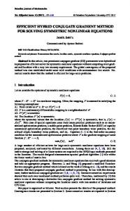
Example 1. We tested the algorithm for the European spread call option pricing problem with the parameters

𝜎1 = 0.2;

where 𝐿 represents the spatial differential operator of (1). If we rewrite (19) in the form

(

In this section we illustrate numerical results for both European and American spread options. In Example 1 we show that the stability conditions (35) and (36) for the European spread option can not be disregarded.

𝑇 = 1;

𝑈 − 𝑔 (𝑆1 , 𝑆2 ) ≥ 0,

𝜕𝑊 − L𝑊 = 0, 𝜕𝜏

7. Numerical Examples

(83)

𝑛 is defined by the finite difference equation (24). where 𝑤𝑖,𝑗

𝑘 < 0.0112.

(85)

These conditions are crucial for the qualitative properties such as positivity and stability of the scheme. In Figure 2 the numerical solution with ℎ and 𝑘 satisfying (85) is presented. On the other hand, in Figure 3 there is a numerical simulation with time step 𝑘 = 0.012 > 0.0112. The solution is unstable and it has negative values. Example 2 illustrates the computational time as well as the comparison with analytical approximation, provided by [6].


9 Table 1: Comparison proposed method (FDM) with analytical approximation (86).

U(S1 , S2 , T)

2500

𝑆2

2000

𝑆1 400 200 100 50 400 200 100 50 CPU time (sec)

1500

100

1000 500 0 −500 1500

90 1000

S1

500 0

0

100

200

300

400

S2

FDM 210.5978 24.2895 0.1150 3.1179𝑒 − 05 220.0678 29.8745 0.1691 5.2150𝑒 − 05 106.188

Approximation 209.7261 23.4543 0.0123 −4.7741𝑒 − 10 220.1714 29.8724 0.0372 −1.9574𝑒 − 09 929.467

Figure 3: Stability condition is broken.

𝑈 (𝑆1 , 𝑆2 , 𝑇) = 𝑆1 𝑒−𝑞1 𝑇 𝑁 (𝑑1 ) − (𝐸𝑒−𝑟𝑇 + 𝑆2 ) 𝑒−(𝑟−̃𝑟−̃𝑞2 )𝑇 𝑁 (𝑑2 ) ,

(86)

400 300 200 100 0 400

0 300

𝑑1 =

𝑆1 1 (ln 𝑆2 + 𝐸𝑒−𝑟𝑇 𝜎√𝑇

+ (𝑟 − ̃𝑟 + 𝑞̃2 − 𝑞1 +

1000

100 0

1500

S1

Figure 4: European spread put option with parameters (84).

𝜎2 ) 𝑇) , 𝑑2 = 𝑑1 − 𝜎√𝑇, 2

2 𝑆2 𝑆2 + ( ) 𝜎22 , 𝜎 = √ 𝜎12 − 2𝜌𝜎1 𝜎2 𝑆2 + 𝐸𝑒−𝑟𝑇 𝑆2 + 𝐸𝑒−𝑟𝑇

(87)

𝑆2 𝑟, 𝑆2 + 𝐸𝑒−𝑟𝑇

𝑞̃2 =

500

200 S2

where

̃𝑟 =

500 U(S1 , S2 , T)

Example 2. Consider the European spread option with the data of Example 1 (84) and choosing step sizes satisfying the stability condition. The price of European spread option can be expressed as the price of a compound exchange option (see [6]). The known derived analytical approximation for the spread option reads

𝑆2 𝑞. 𝑆2 + 𝐸𝑒−𝑟𝑇 2

The comparison of our proposed numerical method and the analytical approximation (86) is presented in Table 1. Analytical approximation is calculated for the same arrays of 𝑆1 and 𝑆2 using MATLAB-function cdf for calculating cumulative distribution function that requires a lot of computational resources, for each point. In the proposed finite difference method (FDM) cdf is only used for the boundary conditions. Last row in the Table 1 presents the CPU time for each method for the same sizes of array. For approximation method cdf-time is 925.018 sec. It is the main

part of computational time. In the case of FDM cdf takes less than half of computational time - 48.867 sec. Furthermore, unsuitable negative values appear in analytical approximation for small 𝑆1 and 𝑆2 while the proposed method preserves nonnegativity of the solution. In the next example we confirm that for the spread put option case the removing technique is fruitful and the selection of the boundary conditions at the boundary of the numerical domain is appropriated because the behaviour of the solution at the boundaries fits the solution at the interior points as it is shown in Figure 4. Example 3. With the parameters in (84) of Example 1, but with payoff (𝑆2 +𝐸−𝑆1 )+ in Figure 4, we show the simulation of the numerical solution obtained by the proposed numerical scheme. Finally, in Example 4 we compare the numerical solution obtained with our scheme (83) using LCP approach with other tested efficient methods presented in [28].

10


Table 2: Comparing several methods for American option pricing. 𝐸 0 2 4

Analytic 8.513201 7.542296 6.653060

FFT 8.513079 7.542242 6.652976

MC 8.516613 7.545496 6.656364

FDM 8.508198 7.534064 6.648792

Example 4. Let us consider the American spread call option problem with parameters:

Table 3: CPU time in sec (first row) and absolute difference (second row) for different methods depending on number of time steps for fixed number of space steps for parameters (89). 𝑁𝜏 50 32 16

𝑇 = 1; 𝜎1 = 0.1;

8

𝜎2 = 0.2;

4

𝑟 = 0.1;

NIM 296.598 0.003 127.069 0.0035 33.493 0.0012 10.360 0.0105 4.117 0.0364

MOL 59.20 0.001 55.12 0.006 51.718 0.0236 49.01 0.074 45.47 0.2512

Monte Carlo 47 970 0.1735 19 811 0.1148 5 149 0.132 1 350 0.1316 355.75 0.1351

FDM 26.547 0.0036 17.911 0.0122 9.432 0.0371 4.787 0.0907 2.815 0.2254

(88)

𝑞1 = 0.05; 𝑞2 = 0.05; 𝜌 = 0.5. Table 2 shows the option price at fixed asset prices 𝑆1 = 96 and 𝑆2 = 100 for different values of strike price 𝐸 evaluated by one-dimensional integration analytic method (Analytic), Fast Fourier Transform (FFT), Monte Carlo (MC) method, and our proposed method. The accuracy is competitive with other methods, such as Fourier Transform with high number of discretization (4096) and Monte Carlo with big number of time steps (2000). Another set of parameters can be considered in order to compare it with data in [9]:

been used in the Monte Carlo method described in [30]. In our method FDM, the step size discretization considered is ℎ = 0.1. To compare FDM with the three previous methods, absolute errors are computed in Table 3 with respect to a reference value obtained by the Fourier space time-stepping approach of Surkov [31] with large number of nodes: 4096 spatial nodes and 300 time steps. From Table 3 we can state that the proposed method has the same order of accuracy as MOL, more efficient, and requires less computational time than Monte Carlo method. It is slightly less efficient than the NIM, but we prove that it possesses a very highly desirable qualitative behaviour in finance.

𝑇 = 0.5;

Competing Interests

𝐸 = 100;

The authors declare that there is no conflict of interests regarding the publication of this article.

𝜎1 = 0.25; 𝜎2 = 0.3; 𝑟 = 0.03;

Acknowledgments (89)

𝑞1 = 0.06; 𝑞2 = 0.02; 𝜌 = 0.5. In [9], three methods are considered to evaluate the spread option price for data 7.4 and fixed values 𝑆1 = 100 and 𝑆2 = 200: a numerical integration method (NIM), a method of lines (MOL), and a Monte Carlo approach. NIM used in [9] is based in the recursive integration techniques developed by Huang et al. [29]. In NIM the option is treated as a Bermudan that is an option that can be exercised at discrete points of time and Simpsons rule is used. For the experiment, the authors used 1024 spatial nodes; see [8, 9] for more details. The MOL is implemented by a spatial discretization of 1438 × 200 mesh points and a three-time level scheme is used for the integration in time [9]. 50 000 simulations have

This work has been partially supported by the European Union in the FP7- PEOPLE-2012-ITN Program under Grant Agreement no. 304617 (FP7 Marie Curie Action, Project Multi-ITN STRIKE-Novel Methods in Computational Finance) and the Ministerio de Econom´ıa y Competitividad Spanish Grant MTM2013-41765-P.

References [1] R. Carmona and V. Durrleman, “Pricing and hedging spread options,” SIAM Review, vol. 45, no. 4, pp. 627–685, 2003. [2] P. P. Boyle, “Options: a Monte Carlo approach,” Journal of Financial Economics, vol. 4, no. 3, pp. 323–338, 1977. [3] C. Joy, P. P. Boyle, and K. S. Tan, “Quasi-Monte Carlo methods in numerical finance,” Management Science, vol. 42, no. 6, pp. 926–938, 1996. [4] W.-H. Kao, Y.-D. Lyuu, and K.-W. Wen, “The hexanomial lattice for pricing multi-asset options,” Applied Mathematics and Computation, vol. 233, pp. 463–479, 2014.

Abstract and Applied Analysis [5] E. Kirk and J. Aron, “Correlation in the energy markets,” in Managing Energy Price Risk, V. Kaminski, Ed., pp. 71–78, Risk Books, London, UK, 1995. [6] C. Alexander and A. Venkatramanan, “Analytic approximations for spread options,” ICMA Centre Discussion Papers in Finance DP2007-11, ICMA Centre, 2007. [7] N. D. Pearson, “An efficient approach for pricing spread options,” The Journal of Derivatives, vol. 3, no. 1, pp. 76–91, 1995. [8] C. Chiarella and J. Ziveyi, “Pricing American options written on two underlying assets,” Quantitative Finance, vol. 14, no. 3, pp. 409–426, 2014. [9] J. Ziveyi, The evaluation of early exercise exotic options [Ph.D. thesis], University of Technology, Sydney, Australia, 2011. [10] P. Boyle, “A lattice framework for option pricing with two state variables,” Journal of Financial and Quantitative Analysis, vol. 23, no. 1, pp. 1–12, 1988. [11] M. Rubinstein, “Return to Oz,” RISK, vol. 7, no. 11, pp. 67–71, 1994. [12] R. Company, L. Jódar, M. Fakharany, and M.-C. Casabán, “Removing the correlation term in option pricing Heston model: numerical analysis and computing,” Abstract and Applied Analysis, vol. 2013, Article ID 246724, 11 pages, 2013. [13] S. Salmi, J. Toivanen, and L. von Sydow, “Iterative methods for pricing american options under the bates model,” Procedia Computer Science, vol. 18, pp. 1136–1144, 2013. [14] J. Toivanen, “A componentwise splitting method for pricing american options under the bates model,” in Applied and Numerical Partial Differential Equations, vol. 15 of Computational Methods in Applied Sciences, pp. 213–227, Springer, 2010. [15] R. Zvan, P. A. Forsyth, and K. R. Vetzal, “Negative coefficients in two-factor option pricing models,” Journal of Computational Finance, vol. 7, no. 1, pp. 37–73, 2003. [16] B. Düring, M. Fournié, and C. Heuer, “High-order compact finite difference schemes for option pricing in stochastic volatility models on non-uniform grids,” Journal of Computational and Applied Mathematics, vol. 271, pp. 247–266, 2014. [17] K. J. in ’t Hout and C. Mishra, “Stability of ADI schemes for multidimensional diffusion equations with mixed derivative terms,” Applied Numerical Mathematics, vol. 74, pp. 83–94, 2013. [18] C. Chiarella, B. Kang, G. H. Mayer, and A. Ziogas, “The evaluation of American option prices under stochastic volatility and jump-diffusion dynamics using the method of lines,” International Journal of Theoretical and Applied Finance, vol. 12, no. 3, pp. 393–425, 2009. [19] M. Fakharany, R. Company, and L. Jódar, “Positive finite difference schemes for a partial integro-differential option pricing model,” Applied Mathematics and Computation, vol. 249, pp. 320–332, 2014. [20] P. R. Garabedian, Partial Differential Equations, AMS Chelsea Publishing, Providence, RI, USA, 1998. [21] D. J. Duffy, Finite Difference Methods in Financial Engineering: A Partial Differential Equation Approach, John Wiley & Sons, Chichester, UK, 2006. [22] R. U. Seydel, Tools for Computational Finance, Springer, 3rd edition, 2006. [23] M. Ehrhardt, Discrete artificial boundary conditions [Ph.D. thesis], Technische Universitat Berlin, Berlin, Germany, 2001. [24] R. Kangro and R. Nicolaides, “Far field boundary conditions for Black-Scholes equations,” SIAM Journal on Numerical Analysis, vol. 38, no. 4, pp. 1357–1368, 2000.

11 [25] J. C. Hull, Options, Futures and Other Derivatives, Prentice-Hall, Upper Saddle River, NJ, USA, 2000. [26] G. D. Smith, Numerical Solution of Partial Differential Equations: Finite Difference Methods, Clarendon Press, Oxford, UK, 3rd edition, 1985. [27] P. A. Forsyth and K. R. Vetzal, “Quadratic convergence for valuing American options using a penalty method,” SIAM Journal on Scientific Computing, vol. 23, no. 6, pp. 2095–2122, 2002. [28] M. A. H. Dempster and S. S. G. Hong, Spread Option Valuation and the Fast Fourier Transform, WP 26/2000, Judge Institute of Management Studies, University of Cambridge, 2000. [29] J.-Z. Huang, M. G. Subrahmanyam, and G. G. Yu, “Pricing and hedging american options: a recursive integration method,” Review of Financial Studies, vol. 9, no. 1, pp. 277–300, 1996. [30] A. Ibán˜ ez and F. Zapatero, “Monte Carlo valuation of American options through computation of the optimal exercise frontier,” Journal of Financial and Quantitative Analysis, vol. 39, no. 2, pp. 253–275, 2004. [31] V. Surkov, “Parallel option pricing with fourier space timestepping method on graphics processing,” in Proceedings of the 1st International Workshop on Parallel and Distributed Computing in Finance (PDCoF ’08), Miami, Fla, USA, 2008.

Advances in

Operations Research Hindawi Publishing Corporation http://www.hindawi.com

Volume 2014

Advances in

Decision Sciences Hindawi Publishing Corporation http://www.hindawi.com

Volume 2014

Journal of

Applied Mathematics

Algebra

Hindawi Publishing Corporation http://www.hindawi.com


Volume 2014

Journal of

Probability and Statistics Volume 2014

The Scientific World Journal Hindawi Publishing Corporation http://www.hindawi.com


Volume 2014

International Journal of

Differential Equations Hindawi Publishing Corporation http://www.hindawi.com

Volume 2014

Volume 2014

Submit your manuscripts at http://www.hindawi.com International Journal of

Advances in

Combinatorics Hindawi Publishing Corporation http://www.hindawi.com

Mathematical Physics Hindawi Publishing Corporation http://www.hindawi.com

Volume 2014

Journal of

Complex Analysis Hindawi Publishing Corporation http://www.hindawi.com

Volume 2014

International Journal of Mathematics and Mathematical Sciences

Mathematical Problems in Engineering

Journal of

Mathematics Hindawi Publishing Corporation http://www.hindawi.com

Volume 2014


Volume 2014

Volume 2014


Volume 2014

Discrete Mathematics

Journal of

Volume 2014


Discrete Dynamics in Nature and Society

Journal of

Function Spaces Hindawi Publishing Corporation http://www.hindawi.com


Volume 2014


Volume 2014


Volume 2014

International Journal of

Journal of

Stochastic Analysis

Optimization



Volume 2014

Volume 2014