An Efficient Method to Estimate Labelled Sample Size for Transductive LDA(QDA/MDA) Based on Bayes Risk Han Liu∗ Department of Computer Science, University of Toronto Email:
[email protected] November 20, 2004 ABSTRACT As semi-supervised classification drawing more attention, many practical semi-supervised learning methods have been proposed. However,one important issue was ignored by current literature–how to estimate the exact size of labelled samples given many unlabelled samples. Such an estimation method is important because of the rareness and expensiveness of labelled examples and is also crucial in exploring the relative value of labelled and unlabelled samples given a specific model. Based on the assumption of a latent gaussian-distribution to the domain, we described a method to estimate the number of labels required in a dataset for semi-supervised linear discriminant classifiers (Transductive LDA) to reach an desired accuracy. Our technique extends naturally to handle two difficult problems: learning from gaussian distributions with different covariances, and learning for multiple classes. This method is evaluated on two datasets, one toy dataset and one real-world wine dataset. The result of this research can be used in areas such text mining, information retrieval or bioinformatics.
∗
For the 15th ECML/PKDD conference
1
1
Introduction
Machine learning falls into two broad categories: supervised learning and unsupervised learning, primarily distinguished by the use of labelled and unlabelled data. Semisupervised learning has received considerable attention in the literature due to its potential in reducing the need for expensive labelled data [1]. A general strategy is to assume that the distribution of unlabelled data is linked to their labels. In fact, this is a necessary condition for semi-supervised learning to work. Existing approaches make different assumptions within this common framework. Generative mixture model method[2] assumes that data comes from some identifiable mixture distribution, with unlabelled data, the mixture components can be identified independently. Transductive Support Vector Machines[3] take the metrics space to be a high-dimensional feature space defined by the kernel, and by maximizing the margin based on the unlabelled data, effectively assume that the model is maximally smooth with respect to the density of unlabelled data in feature space. Co-training[4] assumes that data attributes can be partitioned into groups that individually sufficient for learning but conditionally independent given the class, and working by feeding classifications made by one learner as examples for the other and vice versa. Graph methods[5] assume a graph structure underlying the data and the graph structure coincide with classification goal. The nodes of the graph are data from the dataset, and edges reflect the proximity of examples. The intuition is that close examples tend to have similar labels, and labels can propagate along dense unlabelled data regions. While many practical semi-supervised classification algorithms have been proposed, an important issue is ignored: Given many unlabelled samples, what is the minimum labelled samples we need while achieving a desired classification performance? Given labels to more training samples lowered the classification errors, but increased the cost when obtaining those labels. Thus, a method to estimation the minimum labelled sample size becomes a necessity. Moreover, a detailed analysis of labelled sample size under specific model assumption can improve our understanding of the relative values of labelled and unlabelled samples. In this paper, our labelled sample size estimation method was derived by computing the bays error for a binary semi-supervised linear classifier(i.e. transductive LDA), and estimating the appropriate number of labels necessary for the a certain classification accuracy . We chose transductive LDA in our setting since as a generalization of regular LDA and based on the assumption of a latent gaussian-distribution to the domain,it has a relatively large bias but little variance, and avoid overfitting effectively when sample size is small. Besides a theoretical underpinning, we also developed a computationally tractable implementation based on simple parameter vector space transformation for our estimation method. Detailed discussion and analysis are presented to show that the technique could extend naturally to quadratic classifiers and to multi-class classifiers. The next section provided background information on transductive LDA as discussed in the literature of semi-supervised learning. Section 3 detailed a mathematical derivation of 2
the labelled sample size estimation method for transductive LDA classifiers. Section 4 discussed the extension of our estimation method to the case of quadratic discriminant analysis and multi-class classification. Experimental results on both toy data and real world dataset were shown in Section 5. Summarization and future work were discussed in section 6. the last part was the acknowledge.
2 2.1
Transductive Linear Discriminant Analysis Formalization of Labelled Sample Size Estimation Problem
We begin with a domain of objects X = {x1 , ..., xn }. Each object xi is associated with a vector of observable features(also denoted xi ). We are given labels Yl = {y1 , ..., yl } for the first l objects(l δ1 (x) and class 1 otherwise. With π2 = 1 − π1 , the Bayes risk R∗ is given by 1 1 π1 R∗ = π1 P1 (X T Σ−1 (µ2 − µ1 ) > µT2 Σ−1 µ2 − µT1 Σ−1 µ1 + log ) 2 2 π2 1 π1 1 +π2 P2 (X T Σ−1 (µ2 − µ1 ) < µT2 Σ−1 µ2 − µT1 Σ−1 µ1 + log ) 2 2 π2 In class g1 , X ∼ N (µ1 , Σ), and Z1 = X T Σ−1 (µ2 − µ1 ) is transformation of X and is a univariate Gaussian random variable with mean µ2 − µ1 )T Σ−1 µ1 , and variance σ 2 = (µ2 − µ1 )T Σ−1 (µ2 − µ1 )). Z can be transformed to a standard Gaussian random variable Z−(µ2 −µ1 )T Σ−1 µ1 ∼ N (0, 1). In class g2 , Z has similar distribution except for its mean and σ Z−(µ2 −µ1 )T Σ−1 µ2 ∼ N (0, 1). Thus, the Bayes risk can be calculated as σ π 1 P1 (
Z − (µ2 − µ1 )T Σ−1 µ2 Z − (µ2 − µ1 )T Σ−1 µ1 > a 1 ) + π 2 P2 ( > a2 ) σ σ
where a1 = a2 =
1 T −1 µ Σ µ2 2 2 1 T −1 µ Σ µ2 2 2
− 12 µT1 Σ−1 µ1 + log ππ21 − (µ2 − µ1 )T Σ−1 µ1 −
1 T −1 µ Σ µ1 2 1
σ + log ππ21 − (µ2 − µ1 )T Σ−1 µ2
σ Let Φ denote the cumulative distribution function for a standard Gaussian model. R∗ can π1 π1 1 2 1 2 − σ +log σ +log be written as π1 (1 − Φ( 2 σ π2 )) + π2 Φ( 2 σ π2 ).
3.2
Labelled Sample Size Estimation Method
The estimation of an appropriate size of the labelled samples is determined by the required reduction in R(l, u) − R∗ , which is affected by the current size of unlabelled data,dimensionality of the sample space and the separability of the two classes. We first derive a way to calculate R(l, u)−R∗ . R(l, u) is a function of θ, where θ = (π1 , µ1 , µ2 , Σ−1 )T . We let θ∗ denotes the true value of θ and θˆ denotes the estimated value, and using Taylor ˆ up to second term, we obtain series expansion of R(θ) ˆ = R(θ∗ ) + R(θ)
∂R(θ)T 1 ∂ 2 R(θ)T |θ=θ∗ (θˆ − θ∗ ) + tr{ |θ=θ∗ (θˆ − θ∗ )(θˆ − θ∗ )T } ∂θ 2 ∂θ2
where tr(A) denotes the trace of a matrix A. The term ∂R(θ) | ∗ is zero since θ∗ is an ∂θ θ=θ ˆ = θ∗ ), R(l, u) − R∗ extreme point of R(θ). Assuming the bias of θˆ is negligible, i.e. (E{θ} 5
2 R(θ) ˆ can be approximated as 12 tr{ ∂ ∂θ 2 |θ=θ ∗ cov(θ)}. By asymptotic theory, as the sample size 2 approaches infinity, θˆ ∼ N (θ∗ , J −1 (θ)), where J(θ) = − ∂∂θθl(θ) T , with l(θ) representing the log likelihood of θ, is the observed fisher information matrix of θ, and an approximation ˆ J(θ) is calculated by the summation of two parts: Jl (θ) of the covariance matrix cov(θ). from the labelled data, and Ju (θ) from the unlabelled data. Let n be the total sample size; Jl (θ) and Ju (θ) be the observed information of a single observation for labelled and unlabelled data respectively. If given an required reduction in classification error 4err , we can find the labelled sample size l needed from
tr{
∂ 2 R(θ) ˆ + (n − l)Ju (θ)) ˆ −1 } < 2 · 4err | ˆ(lJl (θ) ∂θ2 θ=θ
(∗)
Since Jl (θ) = Jl (θ)/l0 and Ju (θ) = Ju (θ)/(n − l0 ), where l0 is current labelled sample size, and since n − l ≈ n − l0 (n >> l0 and n >> l), formula (*) can be simplified as follows, ∂ 2 R(θ) ˆ + J2 (θ)) ˆ −1 } < 2 · 4err tr{ |θ=θˆ(lJ1 (θ) 2 ∂θ
3.3
(∗∗)
Computational Consideration
2 R(θ) ˆ ˆ According to formula (*), quantities ∂ ∂θ ˆ, Jl (θ) and Ju (θ) need to be computed first 2 |θ=θ when estimating the desired labelled sample size l. However, when the dimensionality p of the feature space is very large, the computation is very intensive. To illustrate, if R(θ) is a 2 R(θ) 2 2 continuous function,the ∂ ∂θ ˆ is a (p + 5p + 2)/2 × (p + 5p + 4)/2 dimensional matrix, 2 |θ=θ not mentioning the product of two such high-scale matrix! Finding a computationally tractable method to compute formula (**) is therefore of great practical benefit. In this 2 R(θ) section, we develop a method to reduce the computational load of ∂ ∂θ ˆ to a 2 × 2 2 |θ=θ matrix calculation based on simple vector space transformation, while at the same time reduce the matrix production calculation of two (p2 +5p+2)/2×(p2 +5p+4)/2 dimensional matrix production to two 2 × 2 matrix production. According to the proof in [7], in the case of LDA, R(l, u) only depends on π1 and σ 2 (σ 2 = (µ2 − µ1 )T Σ−1 (µ2 − µ1 )) instead of the full parameter set. Let ϕ = (σ 2 , π1 ), and let ϕ∗ denotes the true value of ϕ and ϕˆ denotes the estimation, by Taylor series expansion of R(ϕ) ˆ up to second order, we obtain
R(ϕ) ˆ = R(ϕ∗ ) +
∂R(ϕ)T 1 ∂ 2 R(ϕ)T |ϕ=ϕ∗ (ϕˆ − ϕ∗ ) + tr{ |ϕ=ϕ∗ (ϕˆ − ϕ∗ )(ϕˆ − ϕ∗ )T } 2 ∂ϕ 2 ∂ϕ
Again,the term ∂R(ϕ) | ∗ is zero since ϕ∗ is an extreme point of R(ϕ). If the bias of ϕˆ is ∂ϕ ϕ=ϕ negligible,i.e., (E{ϕ} ˆ = ϕ∗ ), R(l, u) − R∗ can be approximated as, 1 ∂ 2 R(ϕ) R(l, u) − R∗ = tr{ |ϕ=ϕ∗ cov(ϕ)} ˆ 2 ∂ϕ2 The approximated covariance matrix of ϕˆ can be obtained from the inverse of observed ˜ ˜ is the log likelihood of θ˜ based ˜ = − ∂ 2 l(θ) | ˜ θ˜∗ , where l(θ) fisher information matrix J(θ) ∂ θ˜θ˜T θ= 6
on the ladled and unlabel samples. θ˜ is reparameterized from the old parameter θ = (π1 , µ12 , ...µ1p , µ22 , ..., µ2p , aij )T , where aij is the elements of the matrix Σ−1 , i = 1, ..., p,j = 1, ..., p. We map the elements in the original parameter space of θ to the new parameter space θ˜ by letting θ˜ = (π1 , σ 2 , µ12 , ...µ1p , µ22 , ..., µ2p , aij |i,j6=1 )T , i.e., removing the term a11 ˜ from θ and adding the term σ 2 . The vector space of ϕ is a subspace of vector space θ. ˜ Since θ and θ have the same dimensionality, the mapping is guaranteed to be one to one transformation, with a11 expressed by the elements of θ˜ as P σ 2 − i,j6=1 aij (µ1i − µ2i )(µ1j − µ2j ) a11 = (µ11 − µ21 )2 ˜ can be easily obtained from Again aij is the element of Σ−1 . The new log likelihood l(θ) ˜ The information J(θ) ˜ is also the original l(θ) and can be differentiated with respect to θ. ˜ ˜ the summation of two parts: Jl (θ) from the labelled data and Ju (θ) from the unlabelled ˜ and Ju (θ) ˜ be the observed information of a data. We let n be the total sample size, Jl (θ) single observation for labelled and unlabelled data respectively. Similar to the derivation ˜ + Ju (θ) ˜ and thus J −1 (θ) ˜ ≈ (lJl (θ) ˜ + Ju (θ)) ˜ −1 . Let I(l) denotes the ˜ ≈ lJl (θ) above, J(θ) matrix made of the first two columns and first two rows, under our differentiation order of ˜ we can prove that I(l) ≈ cov(ϕ). θ, ˆ The detailed proof is omitted here. After the vector space transformation, given 4err , formula (**) is equivalent to tr{
∂ 2 R(ϕ) |ϕ=ϕˆ (I(l)} < 2 · 4err ∂ϕ2
(∗ ∗ ∗)
which is computationally tractable. From the mathematical derivation above, we can see that the labelled sample size l is determined by several factors. Because the log likelihood is the likelihood for both labelled and unlabelled data, the final l is affected by the number of unlabelled data and also the dimensionality of the sample space. Furthermore, σ 2 and µk determines whether the two classes are easily classifiable, and it is an important factor in our estimation equation.
4
Relax the Strong Assumptions to Transductive QDA and Transductive MDA
4.1
From Transductive LDA to Transductive QDA
In this section, we discuss how to relax the strong assumption of identical covariance in gaussian mixtures by extending Transductive LDA to Transductive QDA. The mod= ification of EM algorithm is trivial, requiring changes only in the M-step, i.e, Σnew k (
P
u ruk (x
u −µ0 )(xu −µ0 )T + k P k
P
u ruk +lk
¯l ¯l T l l l (xk −xk )(xk −xk ) )
. We also need modifications to the estimation 7
method when relaxing the identical covariance assumption. For quadratic discriminant analysis, each class conditional density is modelled as X|G = gk ∼ N (µk , Σk ), and 1 T −1 the discriminant functions are given as δk (x) = xT Σ−1 k µk − 2 µk Σk µk + log πk and G(x) = arg maxk δk (x). In the case of two classes, the corresponding Bayes risk R∗ is −1 −1 −1 π1 1 T −1 1 T −1 T π1 P1 (X T (Σ−1 2 µ2 −Σ1 µ1 ) > 2 µ2 Σ2 µ2 − 2 µ1 Σ1 µ1 +log π2 )+π2 P2 (X (Σ2 µ2 −Σ1 µ1 ) < −1 −1 π1 1 T −1 T (µT2 Σ−1 2 µ2 − µ1 Σ1 µ1 ) + log π2 ). In class g1 , X ∼ N (µ1 , Σ1 ), Z = X (Σ2 µ2 − Σ1 µ1 ) is 2 a univariate gaussian random variable, which is a transformation of X, with the distribu−1 −1 T −1 T −1 T −1 tion, Z ∼ N ((µT2 Σ−1 2 − µ1 Σ1 )µ1 , σ1 ) where σ1 = (µ2 Σ2 − µ1 Σ1 )Σ1 (Σ2 µ2 − Σ1 µ1 ). T −1 T −1 T −1 By defining mean1 = (µT2 Σ−1 2 − µ1 Σ1 )µ1 and mean2 = (µ2 Σ2 − µ1 Σ1 )µ2 , σ2 = −1 −1 Z−mean1 T −1 T −1 ∼ N (0, 1). In class g2 , Z has (µ2 Σ2 − µ1 Σ1 )Σ2 (Σ2 µ2 − Σ1 µ1 ) We have σ1 Z−mean2 similar distribution such that ∼ N (0, 1). Thus, the Bayes risk for QDA can be σ2 calculated as R ∗ = π 1 P1 ( 1
Z − mean1 Z − mean2 > a 1 ) + π 2 P2 ( > a2 ) σ1 σ2
−1 1 T −1 µT 2 Σ2 µ2 − µ1 Σ1 µ1 +log
π1 −meank
2 π2 where a1 = 2 , k = 1, 2. Let Φ denote the cumulative σk distribution function for a standard Gaussian model. R∗ can then be calculated by π1 (1 − Φ(a1 )) + π2 Φ(a2 ). The above method is a theoretical analysis, in fact, after tuning out the covariance matrix Σ1 and Σ2 , we can simply use a very naive method to merge these two different matrices into one single matrix Σcommon = (π12 · Σ1 + π22 · Σ2 )/(π12 + π22 ), which is still a semi-positive definite and can be used instead to apply the estimation technique for Semi-supervised LDA directly. Another important point to note is that without the assumption of identical covariance matrix, R(l, u) does not depend on (σ 2 , π1 ) only. Consequently, our computational tractable approach dose not hold. Yet, one can still use formula (**) to estimate the appropriate size of labelled samples. For a domain with a very flexible distribution but relatively small dimensionality, applying Semi-Supervised QDA would be more suitable.
4.2
From Two-Class Classification to Multi-Class Classification
Some limitations exist when applying transductive LDA to multi-class classification problems, especially when the size of the labelled set is small. In such situation, the EM algorithm may fail if the distribution structure of the data set is unknown. A natural solution in dealing with multi-class classification is to map the original data samples into a new data space such that they are well clustered in the new space, in which case the distributions of the dataset can be captured by simple gaussian mixtures and LDA can be applied in the new space. Transductive Multiple Discriminant Analysis(MDA)[8] used this idea and defined a linear transformation W of the original p1 -dimension data space to a new p2 -dimension space such that the ratio of between-class scatter Sb to within-class scatter Sw is maximized |W T Sb W | in the new space, mathematically, W = arg maxW |W T S W | . suppose x is an p-dimensional w 8
random vector drawn from C classes in the original has a P data space. The kth class T probability Pk and a mean vector µk . thus Sw = C P E[(x − µ )(x − µ ) |c k k i ] and k=1 i PC PC PC T Sb = k=1 Pi (µk − i=1 Pi µi )(µk − i=1 Pi µi ) . The main advantage of transductive MDA is that the data are clustered to some extent in the projected space, which simplifies the selection of the structure of Gaussian mixture models. The EM algorithm for semisupervised MDA can be found in [9]. Because semi-supervised MDA is just another perspective of semi-supervised LDA, our labelled sample size estimation method also applies well in this setting. Assuming there are k classes altogether, the bayes risk is calculated as follows, R∗ = π1 P1 (δ1 < max(δ2 , ..., δk )) + π2 P2 (δ1 < max(δ1 , δ3 , ..., δk )) + · · · · ·+ πi Pi (δ1 < max(δ1 , ..., δi , δi+1 , ..., δk )) + πk Pk (δ1 < max(δ2 , ..., δk−1 )) which can be computed quite efficiently.
5 5.1
Experiments and Results Toy Data of Mixture of Gaussian with Six Components
To illustrate the performance of our estimation method, first we show an example of no obvious practical significance. Consider Gaussian observation (X, Y ) taken from six classes g1 , g2 , ..., g6 . We know that X and Y are Gaussian variables, and we know exactly the means of (X, Y is (µix , µiy ) and variance-covariance matrices is |Sigmai given that the class G = gi . We need to estimate the mixing parameter pi = p(G = gi ). The data is sampled from a distribution with mixing parameter αi . The total number of our data is 900, with dimensionality equals to two, and are divided into 6 classes: 100 data for class g1 , 100 for class g2 ,150 for class g3 ,150 for class g4 ,200 for class g5 and 200 for class g6 . The means and covariance matrices are shown as follows: µ1 = (− 23 , 1/2)T , µ2 = (2, 2)T , µ3 = (− 12 , 52 )T , µ4 = ( 21 , 0), µ5 = ( 31 , −2)T and µ6 = ( 27 , − 21 )T . For their covariance matrices: µ ¶ µ ¶ µ ¶ µ 5 1 ¶ µ ¶ µ 1 1 ¶ 3 12 3 12 3 1 3 1 2 3 3 10 Σ1 : Σ2 : Σ3 : Σ4 : Σ5 : Σ6 : 1 1 1 1 1 1 5 1 1 2 32 1 2 5 5 2 5 2 2 and their mixing parameters π1 = 19 ,π2 = 19 , π3 = 16 , π4 = 61 ,π5 = 29 , π6 = 19 . Based on these information, 900 data were randomly generated. For our experiment, the initial number of the labelled data is 4 for each class. Applying semi-supervised QDA on the data, we obtained a classification result shown in the first plot of figure 1. Given the desired 4err = 0.05, by our algorithm, the estimated labelled data number is 90, thus at least 15 labels are needed for each class. From the first plot in figure 1, it is easy to see that the fitting is not quite good. the shape of the gaussian and the position is quite different from the original figure. plot 2 was generated from 7 labels per class, the fitting is still not good enough. While plot 3 9
5
5
4
4
3
3
2
2
1
1
0
0
−1
−1
−2
−2
−3
−3
−4
−4
−5 −8
−6
−4
−2
0
2
4
6
8
−5 −8
5
5
4
4
3
3
2
2
1
1
0
0
−1
−1
−2
−2
−3
−3
−4
−4
−5 −8
−6
−4
−2
0
2
4
6
8
−5 −8
−6
−4
−2
0
2
4
6
8
−6
−4
−2
0
2
4
6
8
Figure 1: Illustration of the fitting with 4 labels, 7 labels, 15 labels and 22 labels for each class respectively, in this first 2 cases, the number of labelled data is not large enough, thus can not give out enough information for fitting, while in the latter 2 cases,the number of labelled data is enough,the fitting is good, but given more data can not improve the fitting significantly represents the fitting condition with 15 labels for each class, the fitting result is satisfiable; plot 4 is generated with 22 labels for each classes, we can see that the fitting performance does not improve much from the 15 labels case. The classification error for each class is shown in table 1 below: Running for every label size 10 times. The box plot for these 4 conditions are shown in figure 2, From the box plot above, we can see that with the increase number of the labelled data, the overall error rate was reduced significantly at first, but slightly after it exceeds a threshold. Normally, we use 5% as this threshold.
10
Table 1: Classification error for each classes label number 4/class 7/class 15/class error for g1 0.70515 0.47788 0.54221 error for g2 0.77217 0.73579 0.65222 error for g3 0.18903 0.10350 0.14149 error for g4 0.53220 0.60979 0.60518 error for g5 0.17077 0.10841 0.10666 error for g6 0.16513 0.13630 0.10500 overall error 0.35856 0.31040 0.29419
of toy data 22/class 0.55176 0.55411 0.04770 0.57308 0.10176 0.12819 0.28778
Table 2: Classification error for each classes of wine data label number 16/class 20/class 22/class 24/class error for g1 0.08093 0.01281 0.00000 0.01143 error for g2 0.13134 0.04256 0.04887 0.01190 error for g3 0.37941 0.20619 0.08066 0.04138 overall error 0.13646 0.06948 0.04191 0.01980
5.2
Real World Dataset: Wine Recognition Data
In order to test the idea of our estimation method, we applied it to the problem of wine recognition. These data are the results of a chemical analysis of wines grown in the same region in Italy but derived from three different cultivars. The analysis determined the quantities of 13 constituents found in each of the three types of wines[11]. There are 59 data in the class g1 , 71 data in the class g2 and 48 data in the class g3 , with 13 predictors, i.e., the dimensionality is 13. After randomly choosing 16 labelled data for every class, and requiring 4err = 0.05, our estimated number of the labels needed is l = 60, meaning at least 20 labels are need for each class. the classification errors for each class were shown in table 2 above. From which, we can see the data is easily to be fitted by QDA− thus it satisfies the gaussian assumptions well. The computed bayes risk for this data set is about 0.069480.05=0.01948. From the original data set, compute pairwise about the bayes risk R∗ , it’s 0.01966. the result is very close. The box plot for the classification of each class is shown below:
6
Conclusion and Future Extension
We have examined a labelled sample size estimation problem under a specific model, i.e., semi-supervised LDA. Given an additional probability of error 4err of any Bayesian solution to the classification problem with respect to a smooth prior, 4err = R(l, u) − R∗ , 11
0.8 0.6 0.0
0.2
0.4
Classification Error Rate
0.6 0.4 0.0
0.2
Classification Error Rate
0.8
1.0
Mixture of Gaussians (Labeled Sample Size: 44)
1.0
Mixture of Gaussians (Labeled Sample Size: 24)
I
II
III
IV
V
VI
Overall
I
IV
V
VI
Overall
1.0 0.8 0.6 0.0
0.2
0.4
Classification Error Rate
0.8 0.6 0.4 0.0
0.2
Classification Error Rate
III
Mixture of Gaussians (Labeled Sample Size: 130)
1.0
Mixture of Gaussians (Labeled Sample Size: 90)
II
I
II
III
IV
V
VI
Overall
I
II
III
IV
V
VI
Overall
Figure 2: Illustration of the box plot for 4 labels, 7 labels 15 labels and 22 labels per class respectively under the gaussian-distribution domain assumption, we presented a practical labelled sample size estimation method and a computationally tractable approach. Possible extensions and future work are discussed below. This research result could be applied in different semi-supervised learning domain with probability model type 1 [10]. Linear discriminant analysis and logistic regression are two main representatives of these two classes. Our labelled sample size estimation method applies on semi-supervised LDA well, but not on logistic regression. We believe that similar research on logistic regression model would be very meaningful. Based on the detailed analysis for these two types of models, a common labelled sample size estimation framework maybe built and based on this architecture, interesting research topic can be found.
12
0.8 0.6 0.0
0.2
0.4
Classification Error Rate
0.6 0.4 0.0
0.2
Classification Error Rate
0.8
1.0
Wine Recognition Data (Labeled Sample Size: 60)
1.0
Wine Recognition Data (Labeled Sample Size: 49)
I
II
III
Overall
I
Overall
1.0 0.8 0.6 0.0
0.2
0.4
Classification Error Rate
0.8 0.6 0.4 0.0
0.2
Classification Error Rate
III
Wine Recognition Data (Labeled Sample Size: 72)
1.0
Wine Recognition Data (Labeled Sample Size: 66)
II
I
II
III
Overall
I
II
III
Overall
Figure 3: Illustration of the box plot for 16 labels, 20 labels, 22 labels and 24 labels per class respectively
Acknowledgment The authors would like to thank Dr Sam Roweis’s comment and Kannan Achahan’s suggestions. This work is also supported by scholarship from University of Toronto.
References [1] M. Seeger Learning with labeled and unlabeled data, (Technical Report), Institute for Adaptive and Neural Computation, University of Edinburgh, Edinburgh, United Kingdom, pp. 609-616, 2001
13
[2] Kamal Nigam, Andrew Kachites McCallum, Sebastian Thrun, and Tom Mitchell Text classification from labeled and unlabeled documents using EM, Machine Learning, 39(2/3): pp.103-134, 2000 [3] Kristin Bennett and A.Demiriz Semi-supervised support vector machines,Advances in Neural Information Processing Systems (NIPS) [NIPS99] pp1-7. 1999. [4] Avrim Blum and Tom Mitchell Combing labeled and unlabeled data with cotraining,Proc. Of the 1998 Conference on Computational Learning Theory, pp.1-10, 1998 [5] A.Blum and S.Chawla Learning from labeled and unlabeled data using graph mincut,In proc. 17th Intl Conf. on Machine Learning (ICML) ,pp.1181-1188, 2001 [6] Mardia,K., Kent, J. and Bibby,J. Multivariate Analysis, Academic Press. 1979 [7] T.O’Neil. Normal discrimination with unclassified observations, Journal of American Statistical Association, Volume 73, no. 364, pp 821-826, Dec. 1978 [8] R.Duda and P.Hart. Pattern Classification and Scene Analysis, New York: Wiley, 1973 [9] Ying Wu, Qi Tian, Thomas S. Huang. Discriminant-EM Algorithm with Application to Image Retrieval, Technical Report,UIUC,USA 1999 [10] T.Zhang and F.Oles. A probability Analysis on the value of unlabeled data for classification problem., ICML pp.1191-1198 2000 [11] Forina, M.et al, PARVUS. An Extensdible Package for Data Exploration, Classification and Correlation.,Institute of Pharmaceutical and Food Analysis and Technologies, Via Brigata Salerno, Italy.
14