DOI: 10.1784/insi.2009.51.1.36
ELECTRICAL CAPACITANCE TOMOGRAPHY
An efficient nodal Jacobian method for 3D electrical capacitance tomography image reconstruction R Banasiak, R Wajman and M Soleimani
Image reconstruction using Electrical Capacitance Tomography (ECT) requires an accurate inverse model, which is usually computationally expensive especially in three dimensions. A Jacobian reduction method is presented, which uses the nodal Jacobian method rather than an element-based method to reconstruct images without detriment to the final solution. The image reconstruction of an experimental test data has been presented using the new sensitivity map. Keywords: E lectrical capacitance tomography, permittivity mapping, inverse problem, nodal Jacobian.
1. Introduction Electrical Capacitance Tomography (ECT) is a non-invasive and non-destructive imaging technique that uses electrical capacitance measurement at the periphery of an object[1]. Electrodes at the surface of the volume apply electrical potential into the surrounding area and emergent charge is measured at the boundary. The measured data is then used in an electrostatic model to determine the dielectric permittivity properties of the object. Three-dimensional ECT imaging will become an important tool for industrial imaging for process monitoring in the future[5][10]. Much work has gone into the production of accurate forward models to describe the electrostatic forward model[8] and the inverse model to efficiently recover images of the dielectric parameters[6][7]. For the inverse problem, several image reconstruction techniques have been developed[4][9]. The problem of ECT image reconstruction is two-fold: the model to describe the electrical field distribution within the area must be accurate and the inverse problem must be reliable and computationally efficient at estimating the electrical properties within the imaging area. Numerical algorithms based on the Finite Element Method (FEM) for the forward model rely on the accurate definition of the volume and the mesh discretisation must be adequate for the calculation. It has been found that, for an accurate forward model, the FEM mesh resolution must be of a high quality[6]. In this paper we are using a large FE mesh composed of 22,640 nodes and 114,139 elements to discretise the forward model and improve the efficiency of the inverse solution by using a nodal Jacobian. Traditionally, an element-based Jacobian is used[3], the use of a nodal Jacobian will reduce the size of the inverse problem by around five times, providing an important improvement in the application of 3D ECT.
Robert Banasiak is with the Computer Engineering Department, Technical University of Lodz, Lodz, Poland and the Department of Electronic & Electrical Engineering, University of Bath, UK. Radoslaw Wajman is with the Computer Engineering Department, Technical University of Lodz, Poland. Manuchehr Soleimani is with the Department of Electronic & Electrical Engineering, University of Bath, UK. E-mail:
[email protected]
36
2. Forward problem in 3D ECT The forward problem is the simulation of measurement data for given values of excitation and material permittivity distribution and the inverse problem is the imaging result for a given set of measurement data. To solve the inverse problem we need to solve the forward problem. At this stage we assume there is no wave effect and use a low frequency approximation to Maxwell’s equations. In future, a forward model that takes into account the wave effect could be developed but with high computational costs. With high frequency a more complicated model is needed. In a simplified mathematical model, the electrostatic approximation ∇ × E = 0 is taken, effectively ignoring the effect of wave propagation. Let’s take E = –∇u and assume no internal charges, then the following equation holds:
! " #!u = 0 in Ω.................................. (1) where u is the electric potential, ε is dielectric permittivity and Ω is the region containing the field. The electric potential on each electrode is known as: u = Vk on electrode ek. ..............................(2) where ek is the k-th electrode held at the potential Vk. For each excitation pattern one of the electrodes (in turn) is set to a given voltage u=V and the rest are grounded u=0. Using the FEM[6],[7] method we obtain: KU = B ...........................................(3) where the matrix K is the discrete representation of the operator ∇⋅ε∇, the vector B is the boundary condition term and U is the vector of electric potential solution. The total charges on the k-th electrode is given by: "u I k = # ! dx 2 . ....................................(4) "n ek where n is the inward normal on the k-th electrode.
3. A nodal Jacobian approach for 3D ECT A nodal Jacobian approach has been successfully applied to both 3D electrical impedance tomography[2] and 2D ECT[8]. In this paper a nodal Jacobian approach for 3D ECT has been introduced for the first time. Calculation of the nodal sensitivity matrix for 3D ECT tomography can be based on equations expressing energy of electric field accumulated in sensor space. This energy can be calculated as the energy of the capacitor or as the energy of the electric field: WC = 12 U 2C .......................................(5) ! ! WE = 12 # ! ( x, y, z )E ( x, y, z ) $ E ( x, y, z ) d" ................(6) "
where WC is energy accumulated in the capacitor with capacity C and applied voltage U, WE is energy of the electric field E with electric permittivity distribution ε. As both equations describe the same energy they can be combined as follows: 1 2
U 2C =
1 2
!
!
# ! ( x, y, z ) E ( x, y, z ) $ E ( x, y, z ) d" ............(7) "
Insight Vol 51 No 1 January 2009
and consequently:
! 1 C = 2 # ! ( x, y, z ) E 2 ( x, y, z ) d" . ....................(8) U "
The sensitivity of any point j describes the connection between a change in permittivity distribution in that point and the resulting change of the capacity i, as can be expressed by the following equation:
Si, j =
!Ci ........................................(9) !" j
Combining both equations (8 and 9) and omitting the index i, which is connected with the measurement sequence, we can obtain: ! ! $ " (x, y, z)E 2 (x, y, z)d# . ..................(10) 1 # Sj = 2 U !" j It remains to define εj and how it is connected with the function ε (x, y, z). Typically, when we use finite element modelling for ECT, the function ε (x, y, z) is defined that ε (x, y, z) is equal to some constant value inside each element, so equation (10) can be written as: ! 1 S j = 2 # ! j E 2 ( x, y, z ) d" .........................(11) U " This can be expanded as:
where: Si,j – sensitivity value for the j-th voxel described as (x,y,z) while the i-th capacitance measurement Ci between electrodes e1 and e2 was carried out, Ve1 and Ve2 are potentials applied to ! ! electrodes e1 and e2 respectively, Ee1,i (x, y, z) and Ee2,i (x, y, z) are electric field vectors and εj is a permittivity value for the j-th voxel. Let us now define for each element of the FEM mesh the function ε (x, y, z), which does not have a constant value but is defined as ε (x, y, z, εi, εj, εk , εl) where εi, εj, εk , εl are values of permittivity at the element nodes (ie a tetrahedron can be treated as a single mesh element). So we can define a new sensitivity matrix as: 1 U2
and the equation for the sensitivity matrix can be simplified to: Sj =
! 1 N j ( x, y, z ) E 2 ( x, y, z ) d! . ....................(15) U 2 !"
After some transformations this can be expanded as:
si, p, j (voxel) =
! ! E !e,i, j " E !g,i, j Ve "Vg
1 1 (1 , * 3 a p + 3 b p x1 + 8 $% b p (x2 # x1 ) + c p (y 2 #y1 ) + d p (z 2 #z1 ) &' + * * * 1 * 1 *. (16) " det(J) " )+ c p y1 + $%b p (x3 # x1 ) + c p (y 3 #y1 ) + d p (z 3 #z1 ) &' + 12 * 3 * 1 1 * * $ & + d z + b (x # x ) + c (y #y ) + d (z #z ) 1 p 4 1 p 4 1 ' *+ 3 p 1 12 % p 4 *.
where: si, p, j (voxel) – particular sensitivity value for j-th voxel (which represents coordinates x, y and z) that includes the p-th mesh node while the i-th capacitance measurement Ci between electrodes e1 and e2 was carried out, Ve1 and Ve2 are potentials applied to electrodes e1 and e2 respectively, J is a Jacobian matrix ! ! of Cartesian to local coordinates transformations, E !e,i, j and E !g,i, j are electric field vectors calculated when permittivity distribution for a single voxel is based on the permittivity value on its nodes following the equation (14). The total sensitivity value for a single node can be calculated as: l
si, p (node) =
* ! ! " , % # j (x, y, z) &' Ee1,i (x, y, z) ! Ee2,i (x, y, z) () d$/ ,+ $ /. . .(12) 1 j Si, j (x, y, z) = "# j Ve1 !Ve2
Sj =
If we use shape functions for describing ε (x, y, z, εi, εj, εk , εl) we obtain: ! ( x, y, z, ! i , ! j , ! k , ! l ) = N i ( x, y, z ) ! i + N j ( x, y, z ) ! j + N k ( x, y, z ) ! k + +N l ( x, y, z ) ! . (14)
! ! $ " x, y, z, " i , " j , " k , " l E 2 ( x, y, z ) d#
(
)
#
..............(13)
!" j
!s
i, p, j
(voxel) .........................(17)
j =1
Figure 1 shows the sensitivity map for the 32-electrode ECT sensor developed at University of Lodz, Poland. In this 3D system there are four planes of eight electrodes and the sensitivity maps are shown for measurement between various electrodes in different planes. The sensitivity map here shows the equal sensitivity regions between the excitation and measuring electrodes. In order to verify the new sensitivity formula the Jacobian from this sensitivity formula has been tested using experimental data. Figure 2 shows the image reconstruction result using a linear back projection (LBP) algorithm using this new nodal Jacobian matrix.
5. Conclusions In this work we have shown that an efficient Jacobian reduction technique can reduce the computation time and memory requirement of the inversion of the Hessian matrix in the inverse problem without impinging on the qualitative and quantitative accuracy of the reconstructed images. This is particularly important for the reconstruction of images of a large complicated volume with many unknowns where using a fine mesh would usually be computationally inefficient. 6. Acknowledgement
Figure 1. A nodal Jacobian visualisation
The work is funded by the European Community’s Sixth Framework Programme – Marie Curie Transfer of Knowledge Action (DENIDIA, contract no: MTKD-CT-2006-039546). The work reflects only the author’s views and the European Community is not liable for any use that may be made of the information contained therein. 7. References 1.
Figure 2. Sample image reconstruction result (LBP technique)
Insight Vol 51 No 1 January 2009
R A Williams and M S Beck, Process Tomography – Principles, Techniques and Applications, Butterworth-Heinemann, Oxford, p 550, 1995. 2. B Graham and A Adler, ‘A nodal Jacobian algorithm for reduced complexity EIT reconstructions’, International Journal of Information and Systems Sciences, 2(4):453-468, 2006.
37
3. M Soleimani, ‘Sensitivity maps in three-dimensional magnetic induction tomography’, Insight, Non-Destructive Testing and Condition Monitoring, 48 (1), pp 39-44, 2006. 4. M Soleimani and W R B Lionheart, ‘Image reconstruction in three dimensional magnetostatic permeability tomography’, IEEE Trans Magn, Vol 41, No 4, pp 1274-1279, Apr 2005. 5. W Warsito, Q Marashdeh and L-S Fan, ‘Real time volumetric imaging of multiphase flows volume-tomography (ECVT), Proc 5th World Congress on Industrial Process Tomography, Bergen), pp 755-760, 2007. 6. R Wajman, R Banasiak, Ł Mazurkiewicz, T Dyakowski and D Sankowski, ‘Spatial imaging with 3D capacitance measurements’, Measurement Science and Technology, Vol 17, No 8, pp 2113-2118, August 2006. 7. M Soleimani, ‘Three-dimensional electrical capacitance tomography imaging’, Insight, Non-Destructive Testing and Condition Monitoring, Vol 48, No 10, pp 613-617, 2006. 8. R Banasiak, R Wajman and Ł Mazurkiewicz, ‘Application of charge simulation method for ECT imaging in forward problem and sensitivity matrix simulation’, 5th World Congress on Industrial Process Tomography, Bergen, Norway, pp 10991106, 2007. 9. W Q Yang and L Peng, ‘Review of image reconstruction algorithms for electrical capacitance tomography, Part 1: Principles’, Proc International Symposium on Process Tomography in Poland, Wrocław, pp 123-132, 2002. 10. A Romanowski, K Grudzien, R Banasiak, R A Williams and D Sankowski, ‘Hopper flow measurement data visualization: developments towards 3D’, Proc 5th World Congress on Industrial Process Tomography, Bergen, Norway, 2006.
Ultrasonic Flaw Detection for Technicians, 3rd Edition by J C Drury
In the twenty-five or so years since the first edition of ‘Ultrasonic Flaw Detection for Technicians’was published, there have been a number of advances in transducer technology and flaw detection instruments. The gradual acceptance by industry that the sizing of weld defects by intensity drop was not as accurate as had been claimed led to the development of the TOFD technique. Modern digital flaw detectors and computer technology allow far more information to be stored by the operator. The author thus felt that it was time to give the book a thorough review and to try to address some of the advances. The result is this new edition. Available price £25.00 (Non-Members); £22.50 (BINDT Members) from the British Institute of Non-Destructive Testing, 1 Spencer Parade, Northampton NN1 5AA, England. Tel: +44 (0)1604 630124; Fax: +44 (0)1604 231489; E-mail:
[email protected] Order on-line at www.bindt.org Click on ‘Publications’ – ‘Bookstore’
Enquiry No 901-07 38
Insight Vol 51 No 1 January 2009
Insight – Non-Destructive Testing and Condition Monitoring is the Journal of The British Institute of Non-Destructive Testing. Insight was launched in April 1994, replacing the former British Journal of Non-Destructive Testing and incorporating, in quarterly issues, the former European Journal of Non-Destructive Testing. Insight is published monthly and circulated worldwide to more than 65 countries.
FEATURES PROGRAMME 2009 DEADLINES Theme
Editorial copy
Ad Copy Instruction
Ad Material
Jan
Novel applications
14.11.2008
17.11.2008
28.11.2008
Feb
Conference Papers
05.12.2008
08.12.2008
08.01.2009
The Aerospace Industry
15.01.2009
15.01.2009
29.01.2009
Apr
Ultrasonics
12.02.2009
12.02.2009
26.02.2009
May
Thermal and Optical Methods
12.03.2009
10.03.2009
26.03.2009
Jun *
Electromagnetics
14.04.2009
14.04.2009
24.04.2009
Jul
The Rail Industry
14.05.2009
12.05.2009
27.05.2009
Aug
Condition Monitoring
11.06.2009
12.06.2009
25.06.2009
The Oil & Gas Industry
13.07.2009
14.07.2009
24.07.2009
Oct
Radiography
10.08.2009
11.08.2009
21.08.2009
Nov
Ultrasonics
10.09.2009
11.09.2009
24.09.2009
Power Generation
08.10.2009
09.10.2009
22.10.2009
Mar *
Sep *
Dec *
* Euro issue In addition to the above features, each issue includes general news stories affecting the whole industry, and technical articles on a broad range of subjects. Insight contains: q Technical and scientific reviews q Original research and development papers q Practical case studies and surveys q Details of products and services q Newsdesk – contract and marketing news from the industry q NDT Info – the world’s most comprehensive serially published survey of NDT literature
q Technical literature – a comprehensive review of relevant
literature, including the latest international standards and safety information q International Diary – comprehensive listing of information and Calls for Papers concerning relevant events, conferences, symposia and exhibitions q Profiles on personalities and organisations associated with the industry
Each issue embraces matter that is highly relevant to a wide range of readers, including engineers, technicians, academics and scientists, appealing to practitioners and young graduates alike.
Insight Vol 51 No 1 January 2009
39