of simulated annealing as a general method for solving combinatorial optimization problems, we also compare the method with efficient heuristics on.
An Efficient Simulated Annealing Schedule: Implementation and Evaluation Jimmy Lam and Jean-Marc Delosme Report 8817 September 1988
Department of Computer Science, Yale University. Department of Electrical Engineering, Yale University.
Abstract We present an implementation of an efficient general simulated annealing schedule and demonstrate experimentally that the new schedule achieves speedups often exceeding an order of magnitude when compared with other general schedules currently available in the literature. To assess the performance of simulated annealing as a general method for solving combinatorial optimization problems, we also compare the method with efficient heuristics on well-studied problems: the traveling salesman problem and the graph partition problem. For high quality solutions and for problems with a small number of close to optimal solutions, our test results indicate that simulated annealing outperforms the heuristics of Lin and Kernighan and of Karp for the traveling salesman problem, and multiple executions of the heuristic of Fiduccia and Mattheyses for the graph partition problem.
This research was supported by the Army Research Office under contract DAAL03-86-K-0158, by the National Science Foundation under grant ECS8314750, and by the Office of Naval Research under contracts N00014-84-K0092 and N00014-85-K-0461.
1. Introduction
We assume the reader is familiar with the simulated annealing method [12]. The physical analogy on which the method is based suggests that, to achieve good quality results, the system should be kept close t o thermal equilibrium as the temperature is lowered. Most of the practical simulated annealing schedules have been designed following this heuristic. While the first schedules were problem specific, constructed from experiments, schedules of much wider applicability have been derived recently [I], [8], [14]. The starting point in the derivation of these general schedules is an approximate equilibrium criterion that expresses formally when the system is sufficiently close to equilibrium so that the temperature can be lowered. 1 / T, be the inverse temperature a t step n (after a proposed move is either Let s, accepted or rejected) and let z ( s , ) be the average energy of the system, or cost of the current solution, at step n . We consider the system in quasi-equilibrium at inverse temperature s, if it satisfies the relation
where A is a user specified parameter, and ,u(s,) and a(s,) are, respectively, the equilibrium average and standard deviation of the energy at inverse temperature s, [14]. To get good quality results we seek a schedule, called a A-schedule, that lowers the temperature at every step (i.e. sntl 2 s,) while keeping the system in quasi-equilibrium a t all times. Higher quality results can always be obtained by reducing A so that the new A-schedule ensures a closer approximation of equilibrium. However this improvement comes at the expense of increased computation time. For a given value of A and a given move generation strategy (or move selection process), the A-schedule
where pz(s,) is the variance of the actual energy change in one step at inverse temperature s, , is shown in [14] to give at every step the minimum average energy among all A-schedules. Such a schedule is called an efficient A-schedule; there is one such schedule for each move generation strategy. Since the move generation strategy affects only the factor p2(s,) in the efficient Aschedule, if a move generation strategy maximizes pz(s,) for all inverse temperatures s,, the associated efficient A-schedule minimizes the temperature at every step while satisfying the quasiequilibrium condition (1) and hence minimizes the average energy a t every step. The factor p2(s,) cannot be made arbitrarily large. In fact its value is quite restricted and we show in [14], using models for the energy density function (or density of states) and the move generation strategy, that it is uniquely determined once the acceptance ratio po(s,) (the probability that a proposed move is accepted) is known. The substitution of p2(s,) by its expression in terms of po(s, ) gives the final formula for the efficient A-schedules sn+l=sn +
[a] [
4po(s,)(1 - po(sn 1 [snzuz(sn~] (2-po(sn))2
I-
The increment in inverse temperature is the product of three factors. The first, which also appears in the schedules of Aarts and van Laarhoven [l] and Huang et al. [8], reflects what is common to the quasi-equilibrium criteria. The second is the inverse of the specific heat; its
presence is in agreement with the physical intuition that the larger is the specific heat, the slower should be the cooling. The third shows how the temperature decrement is affected by the move generation strategy, through a function of the acceptance ratio only. Since this factor is maximized if the acceptance ratio is equal to 44%, the move generation strategy should be controlled to keep the acceptance ratio constant, equal to that value. The possibility of such a regulation of the acceptance ratio provides a basis for selection between move generation strategies; for instance, if a strategy manages to generate a higher proportion of downhill moves at low temperatures than another strategy, the associated acceptance ratio will not drop as far below the 44% target value and that strategy should be preferred in the low temperature range. The active control of the move generation to regulate the acceptance ratio is an integral part of our schedule, working in concert with the inverse temperature update formula (3). In the next section, a procedure for the estimation and control of the parameters in the schedule is described together with other practical issues. In Section 3, the performance of the schedule is assessed and the performance of simulated annealing as a general combinatorial optimization method is discussed. Finally, concluding remarks are given in Section 4. 2. Estimation and control of simulated annealing p a r a m e t e r s
Since the inverse temperature update formula (3) depends on the acceptance ratio, po(sn), and the variance of the energy, a2(sn), successful application of the schedule requires proper estimation of these quantities. This section is devoted to these estimation problems and to the method of move generation control, which strongly influences the performance of the schedule. 2.1. Estimation of the s t a n d a r d deviation of the energy
In general, the values of po(sn) and a(sn), needed to update the inverse temperature, are not known a priori and must be estimated. Since the acceptance ratio varies slowly from one inverse temperature to another, the ratio of the number of accepted moves to the number of proposed moves in the last T steps, with T between 100 to 1,000, provides a good approximation for the current po. (We have also experimented with a more elaborate scheme for estimating pol as a weighted average of the last few measured ratios, and did not observe any significant difference between the final results of the two methods.) Unfortunately, such a simple procedure cannot be used for the variance of the energy, a2(s ). If the inverse temperature is fixed and the system is in equilibrium, the estimator
where xi is the energy at step i and p(s ) is the average energy, gives an unbiased estimate of u2(s ) provided that p(s ) is known. However p(s ) is not known and worse, the system is never in equilibrium since with the efficient A-schedule the inverse temperature is updated a t every step. Therefore, the preceding formula cannot be used by itself to estimate a2(s). We need an estimator that gives the current value of a2(s ) using measurements made at previous values of the inverse temperature. Such an estimator can be. constructed using the energy density model introduced in [14]. If the energy density function, P ( z ) , were known we could compute the mean and variance of the energy at different inverse temperatures with
and
where
is known as the padition function. However P ( z ) is unknown and, moreover, it is very hard to estimate the parameters of a model of P (x ) on-line. The data gathered up to step n may give a fairly good description of P ( x ) for values of x above and around p(s,) but are too scanty to enable the accurate description of the lower tail of P ( x ) which, as can be seen from the expression of Z (s ), is most important to estimate u2(s ) for s > sn. A fixed model for P (x ), usable at all temperatures, would require a large number of parameters and that sheer number, combined with the scarcity of the data in the lower tail, would make the on-line estimation of these parameters exceedingly difficult. Thus we seek instead a model with a small number of parameters that represents well P ( x ) e - = for s close to the current temperature s,. The price to pay for that smaller number of parameters is that the parameters vary with the temperature; in order to enable parameter estimation this variation should be slow, hence the quality of the model should be sufficiently high, and this imposes a lower bound on how few parameters one can use. The theory developed in [14] suggests a model for which that lower bound turns out to be quite low in practice. The idea is to model the density function Q,( x ) , which is proportional to m e " = , as a weighted sum of gamma density functions
where xo is the global minimum and
For typical problems this model is shown experimentally to be quite satisfactory with M = 0 [14]. The induced model for P (x )e-= is of the same form, with M I N (sn) and b (s, ) replaced by li? = 2 M , N(s,) = 2N (s,) - 1 and T(s,) = 2b ( s n ) [13]. Note that = 0 if M = 0.
M
Using this model we obtain the approximation for the partition function:
There is a whole family of such approximations since, according to the value of the inverse temperature during the annealing process, one would use the model with the corresponding values (s, ) and T(s, ). Evaluation of the integral yields
which can be substituted into the expression for p(s ) in (4) to obtain
Multiplying both the numerator and the denominator of the above expression by (r(s,)+s )n+l, expanding powers of T(s,)+s into powers of s , and grouping terms according to their powers, we arrive at
+
+
there are 2ii? 3 coefficients and only ii? 3 independent variables, namely T ( s , ) , and pi (s,) for i = 0, 1, . . . , the coefficients are not independent of each other for ii? 2 1.) If these coefficients can be found, the variance of the energy, u2(s), can be computed using (5) to get
-(Since b (s,),
z,
Since p(s ) and u2(s ) are obtained from successive derivatives of an approximation to Z (s ), the relative approximation errors can be expected to grow larger as one goes from Z (s ) to p(s ) and then to u2(s ). Unfortunately it is the last element in that chain that interests us. T o appreciate the increase in relative error when going from p(s ) to u2(s ) observe that, if ai (s ) and bi (s ) were known functions, a better estimate of u2(s ) would be found by taking the derivative of the coefficients with respect to s when applying (5) a t s = s n ; hence one source of inaccuracy when employing (7) with the coefficients ai and bi equal to those obtained for the approximation (6) to p(s ) is that the variation of the coefficients is not taken into account. T o circumvent this difficulty we shall merely use (6) and (7) to provide the functional form of p(s ) - x o and u2(s ), as rational functions of s of numerator degrees ii? and 2ii?, respectively, and denominator degrees ii? 1 and 2(ii? I), respectively. The parameter ii? is selected sufficiently large such that the coefficients vary slowly with s, . To simplify the estimation task and also make it less sensitive to modeling assumptions, the coefficients of the two rational functions will be assumed independent within the functions as well as between the functions. By estimating u(s ) independently, without differentiating p(s ), one can get good quality estimates without knowing how the coefficients of the approximation to p(s ) vary with s .
+
+
In order t o estimate the coefficients in the rational model for a2(s ), we use the method of weighted least-squares. First we have to measure u2(si). Given A, we select a r such that p(s ) changes very little for the last r steps. Then, we can use
as the measured average energy of the system a t step j. However, if we went on to use
A ( s n ) = c ( s n ) bi ( s n ) [ l- c ( s n ) x o ] and B ( s n ) = c ( s n ) [ bo ( % )
+
C
( s n ) b i(sn ) x ~ s n I.
(This approximation is valid if I c ( s , ) b l(sn )xo(s - s, ) I 21.00
Table 3: Comparison between the efficient Xschedule with feedback control and Huang's annealing schedule with standard control. The cities are uniformly distributed.
logarithmic schedule, the schedules by Huang el al., and by Aarts and van Laarhoven, based on a preliminary experiment on the traveling salesman problem with 100 to 400 uniformly distributed cities-the coordinates of such a city are a pair of random numbers uniformly distributed in the interval of 0 to 10,000. T o keep the competition fair, we picked one instance of the traveling salesman problem for each problem size and tested the different annealing schedules and heuristics on that same instance. From the test results shown in Table 2, we observe that Huang's annealing schedule performs significantly better than the others; we, therefore, select Huang7s annealing schedule to compete with the efficient A-schedule. We compare the efficient Xschedule and Huang's annealing schedule on the traveling salesman problem with 100 to 400 uniformly distributed cities. The discrepancy in quality of the solutions from both schedules is kept within 0.2% so that the speedup can be measured. The experimental results are displayed in Table 3 in which 6, representing the average quality of the final solution, is the percentage of the average cost above the estimated best cost. This best cost was found by carrying out a sequence of careful annealing executions with the run-time doubled after every few executions until the average cost was stabilized. The speedups associated with a particular 6 as the number of cities increases are shown along each column in Table 3 while the speedups associated with a particular problem size as the cost improves are shown along each row. The speedup is defined as the ratio of the CPU time used by Huang's annealing schedule with standard control t o the CPU time used by the efficient A-schedule with feedback control. Although the efficient A-schedule is 10% slower per move than Huang7s,we still observe a speedup of up to 24 for the 300-city traveling salesman problem! T o isolate the effect of feedback control from the efficient A-schedule, we experimented on both annealing schedules with both controls. The speedups, computed as the CPU time spent by the efficient A-schedule with standard control over the CPU time spent by the same schedule with
Size 100 200 300 400
6 = 3.6% 1.74 1.37 1.94 1.37
Speedup 6 = 2.9% 6 = 2.2% 3.43 3.27 1.75 2.23 3.00 1.76 2.82 1.87
6 = 1.5% 3.87 2.76 5.00 4.90
Table 4: An experiment with move generation control. Comparison between the efficient Aschedule with feedback control and the same schedule with standard control. The cities are uniformly distributed.
Size 100 200 300 400
6 = 3.6% 1.95 2.19 2.55 2.55
Speedup 6 = 2.9% 6 = 2.2% 1.99 2.04 2.02 2.06 2.26 2.36 2.27 2.80
6 = 1.5% 2.21 2.26 2.70 3.01
Table 5: Comparison between the efficient A-schedule and Huang's annealing schedule with feedback control used in both cases. The cities are uniformly distributed.
feedback control, are displayed in Table 4, while the speedups, computed as the CPU time spent by Huang's annealing schedule over the CPU time spent by the efficient Xschedule when feedback control was employed in both cases, are displayed in Table 5. We observe that the use of feedback control speeds up the efficient A-schedule by a factor of up to 5. However, even when the same control method is used with both annealing schedules, the efficient A-schedule still outperforms Huang's by a factor of up to 3. Figure 2a
Figure 2b
Figure 2c
.......... . . . . . . . .
. . . . . . . .
. . . . . . . .
. . . . . . . .
. . . . . . . .
. . . . . . . .
Figure 2d 1
. . . . . . . . . . . . . . . . . . . . . . . . . . . . . . . .
. . . . . . . . . .
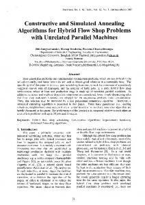
Figure 2: Examples of city distributions for the traveling salesman problem. Figure 2a: 400 uniformly distributed cities. Figure 2b: 256 super-clustered cities (clusters of four). Figure 2c: 100 cities on a lattice. Figure 2d: 100 cities on a lattice with perturbation (up to 50%). We also compare simulated annealing, using the efficient Xschedule and feedback control, with other heuristics for the traveling salesman problem. We chose the heuristics by Lin and Kernighan [15], and by Karp [lo] as the competitors. The comparison with Lin and Kernighan's heuristic covers four types of city distributions: uniformly distributed cities, super-clustered cities, cities on a lattice, and cities on a lattice with small perturbation. In the case of uniformly distributed cities, an instance for each problem size was selected randomly aa the test case. Examples of city distributions are shown in Fig. 2. All results tabulated are the average of at least eight executions. In the case of Lin and Kernighan's heuristic, each execution consists of
three iterations and within each iteration, the local optima found in the preceding iterations are used to speed up the search at the current iteration. The speedups, defined as the ratio of the CPU time used by Lin and Kernighan's heuristic, t', t o the CPU time used by simulated annealing, t , are shown in Table 6 to Table 9. In Table 6 and Table 9, where the optimal costs are not known, 6' and 6 are the percentages above the estimated best costs respectively for Lin and Kernighan's heuristic and for simulated annealing while in Table 7 and Table 8, where the optimal costs are known, 6' and 6 are the percentages above the optimal costs. From these tables, we observe that Lin and Kernighan's heuristic performs very poorly on super-clustered cities and does a very good job on cities on a lattice. This comes a s no surprise since Lin and Kernighan's heuristic produces 3-optimal solutions-an n -optimal solution is a local optimum with respect to moves that exchange n sections of a tour instead of only two sections as in Fig. 1. In the case of super-clustered cities, the number of locally optimal solutions that are 2optimal is large. Therefore, Lin and Kernighan's heuristic spends lots of time going from one 2optimal solution to another until it reaches a boptima1 solution. In the case of cities on a lattice, the number of globally optimal solutions is large: any tour formed by connecting cities either vertically or horizontally is a globally optimal solution. Consequently, the probability of finding one of these optima1 solutions is high and the heuristic terminates quickly.
Size 100 200 300 400
CPU t i m e (sec.) t t'/ t 1' 69.8 296.0 686.1 1492.7
52.9 101.6 197.5 330.8
1.32 2.91 3.47 4.51
Tour l e n g t h 6(%) 6'(%) 1.01 1.25 1.32 1.46
1.01 1.21 1.32 1.40
Table 6: Comparison with Lin and Kernighan's heuristic on the traveling salesman problem for uniformly distributed cities. Size 64 128 256 512
CPU t i m e (sec.) 2' 57.9 428.2 2113.6 13883.1
1
9.3 17.4 61.5 296.3
2'/ t 6.23 24.61 34.37 46.85
Tour l e n g t h 6'(%) 0.58 1.13 2.52 4.11
6(%) 0.58 1.06 2.58 4.03
Table 7: Comparison with Lin and Kernighan's heuristic on the traveling salesman problem for super-clustered cities. Size 100 200 300 400
CPU t i m e (sec.) t t t t' 13.0 70.7 190.3 415.6
78.2 492.0 1338.4 3125.5
0.17 0.14 0.14 0.13
Tour l e n g t h at(%) a(%) 0.20 0.15 0.10 0.25
0.31 0.67 1.09 1.09
Table 8: Comparison with Lin and Kernighan's heuristic on the traveling salesman problem for cities on a lattice.
T o check that the number of globally optimal solutions influences the speed of Lin and Kernighan's heuristic, we perturb the coordinates of the cities on a lattice by up t o P percent of the normal inter-neighbor distance so that the number of globally optimal solutions is small. The new coordinates of a city (XI, y ' ) are computed from the old coordinates (x , y ) according to ( ~ ' 1Y ? = (x
1
Y )
+ MP(~,,ty)
where Mp is P % of the inter-neighbor distance and t, , ty are uniformly distributed random numbers between -1 and 1. The test results for a 200-city problem with different perturbation levels are shown in Table 9 . We observe that the CPU time spent by Lin and Kernighan's heuristics increases from 7 1 seconds to 181 seconds with only a 5% perturbation, but does not increase further with larger perturbations. This observation confirms our conjecture that the abundance of globally optimal solutions speeds up Lin and Kernighan's heuristic. We also experimented with different numbers of cities on a lattice with up to 50% perturbation. As expected, the speedups shown in Table 10 fall in between those for the uniformly distributed cities and the cities on a lattice. In contrast to Lin and Kernighan's heuristic, simulated annealing is relatively insensitive to the structure and regularity of an optimization problem; the CPU time spent by simulated annealing for different city distributions stays fairly constant for a given quality of solution. This combination of the insensitivity of simulated annealing towards the structure of a problem and the sensitivity of Lin and Kernighan's heuristic towards the number of global optima and the number of 2-optimal solutions explains the drastic speedup (up to 46) for problems with superclustered cities as well as the superiority of Lin and Kernighan's heuristic over simulated annealing on problems with cities on a lattice. As mentioned earlier, only one instance for each problem size was chosen for uniformly distributed cities to obtain the test results shown in Table 6 . In order t o check that similar
0% 5% 10% 20% 50%
C P U t i m e (sec.) t' 1 t / t 0.14 70.7 492.0 0.37 180.8 491.1 0.36 179.2 491.1 0.52 154.6 297.2 182.3 205.6 0.89
Tour l e n g t h 6(%) 6'(%) 0.15 0.67 0.21 1.79 0.33 2.27 0.67 0.72 0.73 0.70
Table 9: Comparison with Lin and Kernighan's heuristic on a 200-city traveling salesman problem for cities on a lattice with up to P percent perturbation. Size 100 200 300 400
C P U t i m e (sec.) t t /t 0.31 32.7 104.9 0.89 182.3 205.6 1.89 510.6 270.8 2.34 978.8 417.5
t
Tour l e n g t h 6(%) 6'(%) 0.70 0.70 0.73 0.70 1.42 1.38 1.43 1.42
Table 10: Comparison with Lin and Kernighan's heuristic on the traveling salesman problem for cities on a lattice with up to 50% perturbation.
speedups can be expected for any random instance, we carried out the following experiment. We first randomly picked eight instances of a 200-city traveling salesman problem. Then, Lin and Kernighan's heuristic was used to solve each instance once, resulting in a total of eight executions. Let us refer to these eight executions as a group. Since the CPU time spent by Lin and Kernighan's heuristic is controlled by the number of iterations, we can vary the number of iterations to obtain different groups. Similarly, we can obtain different groups of executions for these eight instances using simulated annealing by controlling the value of A and, hence, the CPU time. The speedups obtained are similar to those shown in Table 6 [13]. Except for the case of cities on a lattice, simulated annealing offers a substantial speedup over Lin and Kernighan's heuristic for high quality solutions. This observation indicates that for problems where globally optimal solutions are sparse and high quality solutions are desired, simulated annealing coupled with a good move generation strategy is an efficient and highly competitive method. Lin and Kernighan's heuristic is only good for small problems since its computation time becomes unacceptable for large problems. Karp designed a heuristic that handles large problems. The comparison with Karp's heuristic was performed on a traveling salesman problem with 10,000 cities whose coordinates are integers uniformly distributed in the interval of 0 t o 1,000,000. Karp's heuristic consists of three stages: partition a problem into M smaller size sub-problem, solve the sub-problems using another heuristic, and patch the resulting solutions to form a tour. In this experiment, we used three iterations of Lin and Kernighan's heuristic to solve the partitioned sub-problems. Two modifications are needed in order for simulated annealing to run on a 10,000-city traveling salesman problem. Ideally, we would like to let M = 9,999 and perform table lookup for the distances between cities. This is, however, impossible due to the 0 (N') storage requirement. As a result, we compute the distances as the need arises and store the distances of only 250 nearest neighbors. The result of the comparison between simulated annealing and Karp's heuristic is shown in Table 11 while the pictures of tours obtained via both methods are shown in Fig. 3. The estimated best cost for this problem is based on the formula [3] lim -= 0.749, ~ - ~ m where Cw is the optimal tour length and I = 1,000,000 is the interval from which the
128 64 32
CPU t i m e (sec.) tl/t t1 t 0.44 4850 11050 0.64 10330 16070 1.22 26460 21610
Tour l e n g t h bl(%) 6(%) 6.98 6.66 3.52 3.41 2.03 1.97
Table 11: Comparison with Karp's heuristic coupled with Lin and Kernighan's heuristic on the traveling salesman problem with 10,000 uniformly distributed cities. In this table, M is the number of sub-problems in the partition, t' and t represent the CPU time for Karp's heuristic and simulated annealing, respectively, while 6' and 6 represent the percentages above the best cost estimated from formula (20). These are the average results of four executions.
coordinates of the cities are picked. Table 11 is constructed by varying the number of partitions used in Karp's heuristic and comparing the resulting solutions with simulated annealing for different values of A. Figure 3a
Figure 3b
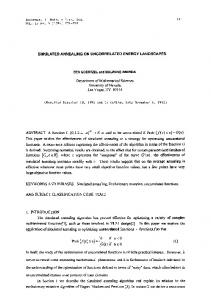
Figure 3: Tours of a 10,000-city traveling salesman problem. Figure 3a: Tour found using simulated annealing, with length 7.59~10'. Figure 3b: Tour found using Karp's heuristic, with length 7 . 6 4 ~lo7; the edges of the 64 squares in the partition can be made out from the tour.
From this table we observe that simulated annealing out-performs Karp's heuristic for high quality solutions. This evidence strongly supports our belief that an efficient annealing schedule coupled with a good move generation strategy makes simulated annealing an extremely effective method. 3.2. Graph partition problem
The graph partition problem (or graph partitioning) is NP-complete 161. The goal of this problem is to partition the vertices of a graph into two equal size vertex sets, VA and VB, so as to minimize the number of edges with end-points in both sets. We first describe the implementation details of the move generation strategy for simulated annealing, followed by a discussion of the test results. Our results are similar to those obtained by Johnson et al. [9] with one essential difference: by using the efficient A-schedule and a good move generation strategy, we are able to speed up simulated annealing significantly. Thus, for the same high quality solution, the CPU time spent by simulated annealing compares favorably with the CPU time spent by multiple executions of Fiduccia and Mattheyses's heuristic [5]. The first part of the discussion covers the comparison between the efficient A-schedule and Huang's annealing schedule while the second part covers the comparison between simulated annealing and Fiduccia and Mattheyses's heuristic. 3.2.1. Implementation details
The cost t o be minimized in a graph partition problem is the size of the cutset-the number of edges with end-points in both vertex sets. In order to increase flexibility in move generation, we follow the suggestion of Johnson et al. and introduce an additional imbalance factor into the cost function:
Cost = cutsize
+