This paper presents a general annealing schedule which speeds ... temperature schedule called simulated annealing schedule (or annealing schedule in short), ...
An Efficient Simulated Annealing Schedule: Derivation Jimmy Lam and Jean-Marc Delosme Report 8816 September 1988
Department of Computer Science, Yale University. Department of Electrical Engineering, Yale University.
Abstract The popularity of simulated annealing comes from its ability to find close to optimal solutions for NP-hard combinatorial optimization problems. Unfortunately, current implementations of the method usually require massive computation time. This paper presents a general annealing schedule which speeds up simulated annealing significantly when compared with general schedules available in the literature. The annealing schedule, which lowers the temperature at every step and keeps the system in quasi-equilibrium at all times, is derived from a new quasi-equilibrium criterion. For a given move generation strategy, this schedule is shown to give the minimum final average cost among all schedules that maintain the system in quasi- equilibrium. An alternate form of the schedule is derived that explicitly relates move generation to temperature decrement. This leads to a control method for the move generation strategy that further minimizes the final average cost.
This research was supported by the Army Research Office under contract DAAL03-86-K-0158, by the National Science Foundation under grant ECS8314750, and by the Office of Naval Research under contracts N00014-84-K0092 and N00014-85-K-0461.
1. Introduction
The ground states of a solid can be reached by heating it up to some high temperature and then cooling it down slowly. This process, called annealing, lets the system settle into a low energy state without getting trapped in a local minimum. By identifying the cost function in a combinatorial optimization problem with the energy of a physical system and the solution space with the system state space, close to optimal solutions can be found via a simulated annealing of the associated system. This method, proposed by Kirkpatrick et al. [9], explores the solution space of the optimization problem by a controlled hill climbing search whose control parameter, T , is the analogue of the temperature. By slowly lowering T towards zero according to a properly chosen schedule, one can show that the set of globally optimal solutions is approached asymptotically, see e.g. [6]. In a typical implementation of simulated annealing [9], the initial temperature is set sufficiently high. A new state (or solution) is generated incrementally from the current state by randomly selecting and proposing a move from a set of predefined moves. A move is a perturbation whose application t o the current state leads to a new state. We shall call the move selection process the move generation strategy. Let the energy (or cost) of the current state be x and the energy of the proposed new state be x,, . The probability that a proposed move is accepted or rejected is determined by the Metropolis criterion [13]:
where Ax = xp - x is the proposed energy change and p ( A x ) denotes the probability of accepting that move. If a proposed move is accepted, time is incremented and the proposed state becomes the current state. If a proposed move is rejected, time is also incremented but the current state remains unchanged. By controlling the temperature T , we control the probability of accepting a hill climbing move (a move that results in a positive A x ) and, therefore, the exploration of the state space. This process of selecting and proposing a move is repeated until the system is considered in thermal equilibrium. Then, the temperature is reduced according to a temperature schedule called simulated annealing schedule (or annealing schedule in short), and the system is allowed to reach thermal equilibrium again. The system is considered frozen and the process is terminated when no significant improvement is expected by further lowering the temperature. At this point, the current state of the system is the solution to the optimization problem. Note that as the temperature is lowered, the exploration of the state space is changed gradually from random-all proposed moves are accepted a t T = m-to greedy---only downhill moves are accepted at T = 0. Since its introduction, simulated annealing has been applied to optimization problems in diverse areas, spanning computer-aided IC design [15], image restoration [5] and code design [4]. This popularity comes from its ability to find close to optimal solutions for NP-hard combinatorial optimization problems. However, its massive requirement of computation time still hinders its application. This paper tackles this problem by optimizing the simulated annealing schedule. In the remainder of this section, we discuss the main approaches employed to develop annealing schedules. (Refer to [lo, Chapter 51 for an extensive survey of different annealing schedules.) For ease of presentation, we define the inverse temperature s as s 1 / T . Time (or step) is discrete and is incremented whenever a proposed move is either accepted or rejected. Furthermore, the inverse temperature is assumed to be a non-decreasing function of time,
sn+k 2 s n 1
k 2 11
where s, is the inverse temperature at step n .
1.1. Logarithmic schedule The analysis of simulated annealing based on time-inhomogeneous Markov chains has been carried out in [5], [6] and [14] among others. This analysis determines constraints on s n , n 2 0, that ensure convergence to globally optimum solutions. A particular schedule is defined by the sequence of inverse temperatures that satisfy these constraints tightly. Let xi be the energy of state i , wi (n ) be the probability that the system is at state i a t step n , and gi,j be the probability of proposing a move from state i to state j. Since the probability that a move from state i to state j is accepted is determined by the Metropolis criterion, p (xj-xi) = min(1, e
-.(I.
' - Z ; ) 1,
the one-step transition probability from state i to state j at step t is
If a proposed move is rejected, the system remains in the same state. Therefore, the probability of staying at state i is
In matrix notation, the probability vector of the system at step n is
W ( n ) = P ( n ) P (n-1)
,
. - P ( 1 ) W (0),
(5)
where W (n ) is a column matrix with elements wi (n ) and P (t ) is a square matrix with elements p,,,(t ). The preceding relation for a time-inhomogeneous Markov chain ( P ( 2 ) is a function of time) is a precise mathematical model for simulated annealing. Using this model, the system may be shown to converge asymptotically with probability 1 to the set of globally optimal solutions if the inverse temperature is changed according to the following schedule:
where X >
l~glo(~(~ 5.81
Qs (2
Figure 3a 1
Points of measurements (z
Qs
>
(z 72
Qs
>
N
=
At point A 147, c = 3.65e-04
=
Qs (z )
Fiqure 3c
N
Figure 3b
At point B 61, c = 4.22e-04
Fisure 3d
N
=
(I ) 16
Figure 3e
At point C 18, c = 6.56e-04 Figure 3f
Qs
60 12 48 08
36 24
04 12 0 7.9
5
0 8.1 8.3 8.5 8.7 8 . 9 ~ 1 0 ~ 47.9 At point D N = 14, c = 2.21e-03 N
=
At point E 28, c = 1.07e-02
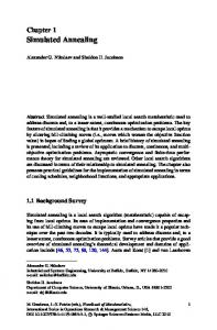
Figure 3: Test results for Q,( I ) at different values of s for a 100-city traveling salesman problem. The inverse temperatures at which the tests were performed are indicated in Figure 3a while the measured Q,(x) (histograms) and the fitted gamma density functions (curves) with parameters N and c are shown in Figure 3b to Figure 3f.
5. Conclusions
The increment in inverse temperature in the efficient A-schedule can be decomposed into three factors:
The first factor, which depends on the quasi-equilibrium criterion, is the same as the factors in Aarts's and Huang's annealing schedules. The second factor relates the specific heat, which is the rate of change of the equilibrium average energy with respect to the temperature,
to the temperature decrement. The presence of this factor is in agreement with the common belief that the larger is the specific heat, the slower should be the cooling. The third factor relates the acceptance ratio and, hence, the move generation strategy to the temperature decrement. As mentioned earlier, to maximize this factor, the move generation strategy should be controlled in order to arrive at a desired acceptance ratio of 44%. This is similar to the suggestion made by Binder [2, p. 111 on Monte Carlo methods in statistical physics that the magnitude of the proposed energy change should be chosen such that the acceptance ratio is close to 50%. Thus, not only the dynamics of the system is accounted for by our annealing schedule, but also the move generation strategy is actively controlled. In [ll], we discuss practical aspects of applying the efficient A-schedule, including parameter estimation and move generation control, and assess the performance of the efficient A-schedule by comparing it with the annealing schedules surveyed in the introduction. Furthermore, we evaluate the performance of simulated annealing as a general combinatorial optimization method by comparing it with other problem specific heuristics on some classical combinatorial optimization problems. References [I]
E. Aarts, and P . van Laarhoven, "Statistical Cooling Algorithm: A General Approach to Combinatorial Optimization Problems," Philips J. of Research, Vol. 40, No. 4, 193-226, 1985.
[2]
K. Binder, Monte Carlo Methods in Statiscal Physics, 2nd Edition, Springer-Verlag, 1986.
[3]
L. Cooper and M. Cooper, Introduction to Dynamic Programming, Pergamon Press, 1981.
[4]
A. El Gamal, L. Hemachandra, I. Shperling, and V. Wei, "Using Simulated Annealing to Design Good Codes," IEEE Trans. Information Theory, Vol. 33, No. 1, 116-123, 1987.
[5]
S. Geman, and D. Geman, "Stochastic Relaxation, Gibbs Distributions, and the Bayesian Restoration of Images," IEEE Trans. Pattern Analysis and Machine Intelligence, Vol. 6 , 721-741, 1984.
[6]
B. Hajek, "A Tutorial Survey of Theory and Applications of Simulated Annealing," Proc. of the 24th IEEE CDC, 755-760, 1985.
[7]
M. Huang, F. Romeo, and A. Sangiovanni-Vincentelli, "An Efficient General Cooling Schedule for Simulated Annealing," Proc. of the IEEE ICCAD, 381-384, 1986.
N. Van Kampen, Stochastic Processes in Physics and Chemistry, North-Holland, 1981. S. Kirkpatrick, C. Gelatt Jr., and M. Vecchi, "Optirnization by Simulated Annealing," IBhf Research Report, RC 95'55, 1982. P . van Laarhoven, and E. Aarts, Simulated Annealing: Theory and Applications, D. Reidel Publishing Company, 1987. J . Lam, and J.-M. Delosme, "An Efficient Simulated Annealing Schedule: Implementation and Evaluation," Technical Report 8817, Department of Electrical Engineering, Yale University, 1988. J . Lam, "An Efficient Simulated Annealing Schedule," Ph.D. Dissertation, Department of Computer Science, Yale University, 1988.
M. Metropolis, A. Rosenbluth, M. Rosenbluth, A. Teller, and E. Teller, "Equation of State Calculations by Fast Computing Machines," J. of Chemical Physics, Vol. 21, 1087-1092, 1953.
D. Mitra, F. Romeo, and A. Sangiovanni-Vincentelli, "Convergence and Finite-time Behavior of Simulated Annealing," Proc. of the 24th IEEE CDC, 761-767, 1985. C. Sechen, and A. Sangiovanni-Vincentelli, "The Timberwolf Placement and Routing Package," IEEE J. of Solid-State Circuits, Vol. 20, No. 2, 510-522, 1985. S. White, "Concepts of Scale in Simulated Annealing," Proc. of the IEEE ICCD, 646-651, 1984.