1
An Efficient Spatial Domain Technique for Subpixel Image Registration Irene G. Karybali, Emmanouil Z. Psarakis, Kostas Berberidis and Georgios D. Evangelidis Dept. of Computer Engineering and Informatics, University of Patras, 26500 Rio-Patras, Greece emails:{karybali, psarakis, berberid, evagelid}@ceid.upatras.gr phone: +30 2610 996969, fax: +30 2610 996971
Abstract In this paper a new technique for performing image registration to subpixel accuracy is presented. The proposed technique, which is based on the maximization of the correlation coefficient, does not require the reconstruction of the intensity values and provides a closed-form solution to the subpixel translation estimation problem. Moreover, an efficient iterative scheme is proposed, which reduces considerably the overall computational cost of the image registration problem. This scheme properly combined with the subpixel accuracy technique results in a fast spatial domain technique for subpixel image registration.
Keywords: Fast image registration, subpixel accuracy, correlation coefficient.
Corresponding Author: Emmanouil Z. Psarakis Dept. of Computer Engineering & Informatics School of Engineering University of Patras 26500 Rio - Patras GREECE E-mail:
[email protected] Tel: +30-2610-996969 Fax: +30-2610-996971
July 26, 2007
DRAFT
2
I. I NTRODUCTION Many image processing applications require an image registration scheme in order to estimate the underlying correspondence between two or more images, which have been acquired either by a single sensor at different times, or by different sensors at the same time but from different viewpoints, or by a combination of the above. Two examples of such applications are remote sensing and biomedical imaging. For remote sensing, registration of infrared to visible spectra is very important for studying satellite images of the earth. Registration is also very useful for the medical community, since can lead to substantially enhanced diagnosis, in surgical planning, or in the comparison of images from different modalities. Many techniques have been proposed for image registration. Two basic categories are the featurebased and the intensity-based techniques [1], [2]. Feature-based techniques first identify edges, contours or other features common to the compared images and then find the mapping between them [3], [4], [5]. This results in reduced computational complexity. However, the problem of identifying features is rather complicated and these techniques are very sensitive to the accuracy of the feature extraction stage. On the other hand, intensity-based techniques are more computationally demanding, but avoid the difficulties of feature extraction. Some typical criteria for intensity-based registration are the minimization of the squared error between the compared images, the correlation maximization [6] and the maximization of mutual information, [7], [8], [9]. The so-called phase-correlation technique, [10], and other Fourier-based [11], [12], as well as wavelet-based techniques, [13], have also been proposed. Some of the referenced methods obtain pixel-level registration that may be adequate for some applications. On the other hand, there are applications that require registration with subpixel accuracy. The most commonly used methods that provide subpixel accuracy are based on interpolation [14]. Some examples are the intensity, the correlation and the phase-correlation interpolation. However, the accuracy of these methods depends highly on the interpolation algorithms’ performance. Other approaches, which do not include interpolation, are based on the differential properties of the image sequences [14], or formulate the subpixel registration as an optimization problem [15], [16], [17]. These approaches rely on the image intensity conservation assumption. In [15], an algorithm for registering multiple frames simultaneously using nonlinear minimization in frequency domain is described, based on the assumption that the original image is bandlimited. The authors of [16] propose a frequency domain technique for registration of aliased images. Their technique is based on spectrum cancellation, that is, elimination of the aliased frequency components. Reddy and Chatterji in [12] use the so-called phase correlation of the log-polar transform of
July 26, 2007
DRAFT
3
the images and apply a high-pass emphasis filter to strengthen high frequencies in the estimation. Another Fourier-based algorithm for image registration with subpixel accuracy is presented in [18], where the pure translation case is investigated. The algorithm detects and removes the frequency components that might cause errors in the shift estimation due to aliasing. In [19], it is shown that the signal power in the phase correlation corresponds to the polyphase transform of a filtered unit impulse centered at the point of registration. More recently, in [20] a frequency domain technique has been proposed for the registration of aliased images, based on their low-frequency, aliasing-free (or marginally affected by aliasing) part. The phase difference between the compared images is computed and for the aliasing-free frequencies the corresponding linear equations are written. Then, the shift parameters are found as the least squares solution of these equations. It is easier to describe and handle aliasing in frequency domain, but frequency domain methods are more suitable for global motion models. On the other hand, spatial domain methods generally allow for more general motion models. In [21], an iterative scheme based on Taylor expansions is presented and a pyramidal scheme is used to increase the precision for large motion parameters. The authors of [22] use sparsely sampled regional correlation, providing accuracy better than 0.2 pixels. In [23], an error function linear in the model (local affine) parameters is minimized using least-squares. This error function is then augmented with a nonlinear smoothness constraint, and the least-squares solution is used to bootstrap an iterative nonlinear minimization. This entire procedure is built upon a differential multiscale framework, allowing the capture of both large- and small-scale transformations. The technique proposed here has been motivated by the approach suggested recently in [24], [25] where an enhanced correlation-based method for stereo correspondence was presented. Based on this work, we present here a spatial domain technique which is suitable for subpixel image registration. The proposed technique aims to maximizing the correlation coefficient, which is a measure that provides robustness to photometric distortions. In contrast to the interpolation based techniques, the proposed one does not require the reconstruction of the intensity values and provides an easily computed closed-form solution. Moreover, an efficient iterative scheme is proposed, which reduces considerably the overall computational cost of the image registration problem. This scheme properly combined with the subpixel accuracy technique results in a fast spatial domain technique for subpixel image registration. Note that if exhaustive search is used for the maximization of the correlation coefficient, N 2 searches are required, where N is the number of searches in each dimension. Using the proposed scheme for the computation of the correlation coefficient function, the number of searches is in most cases much smaller than N 2 . Note that we deal here only with translation, since this is the most costly part of an image registration July 26, 2007
DRAFT
4
problem. However, the proposed technique can be extended so as to cope with other distortions, as well [26]. The paper is organized as follows. In Section II the problem is formulated and the proposed measure along with the closed-form solution are given. In Section III experimental results that evaluate the performance of the proposed subpixel registration technique and compare it to other techniques are provided. The new iterative scheme and some experiments concerning its complexity are presented in Section IV. Finally, the work is concluded in Section V. II. S UBPIXEL I MAGE R EGISTRATION A. Problem Formulation Let f (i, j) be a reference image and w(i, j) a window in f (i, j), with dimensions n × n and with its support defined by the set S = [0, n − 1] × [0, n − 1].
(1)
Let also g(i, j) be a search area in a translated version of image f (i, j), ft (i, j), with dimensions m × m (where m > n). For both w(i, j) and g(i, j), the upper left corner is located at the origin of a global coordinate system. Then, it is clear that all the possible positions of window w(i, j) in the search area g(i, j) take values in the following set A = [0, N − 1] × [0, N − 1],
N =m−n+1
(2)
and their maximum number is upper bounded by the cardinality of set A, i.e., N 2 . Let now sx (i, j) be a window of the search area g(i, j) that has the same size with w, with x = [x, y]t ∈ A, (i, j) ∈ S denoting the coordinates of its upper left corner, and the relative coordinates of
the pixels of the window with respect of its upper left corner respectively. Then, the image registration problem can be stated as a searching problem. Namely, we are searching for a x0 ∈ A such that the following n2 relations hold sx0 (i, j) = w(i, j),
∀(i, j) ∈ S.
(3)
In order to achieve our goal, we need to use an appropriate similarity measure. Such a well known measure is the correlation coefficient of windows w(i, j) and sx (i, j), which is defined as e te Cx = w sx
(4)
e = w/||w|| where w ¯ and e sx = ¯ sx /||sx || stand for the zero mean Euclidean normalized versions of
vectors w ¯ ≡ vec (w(i, j) − mw ) and ¯ sx ≡ vec (sx (i, j) − msx ), with (i, j) ∈ S , mw and msx denoting July 26, 2007
DRAFT
5
the mean values of windows w(i, j) and sx (i, j) respectively, and operator vec stacking each window’s columns in a column vector of length n2 . The correlation coefficient defined in (4) has the advantage of being invariant to linear photometric distortions. This property is required by many image registration applications where the illumination of the scene is nonuniform. Having defined the desired similarity measure by (4) and assuming that the translation differences between the compared windows are constant, we have to compute the correlation coefficient for all the possible positions of the window w(i, j) in the search area g(i, j), in order to find the translation x0 that maximizes (4). In fact, we have to solve the following maximization problem max C x .
x ∈A
(5)
Solving the above defined optimization problem, we can register images with pixel accuracy. However, in many applications sub-pixel accuracy is required [20], [22], [23], [24], [25]. To this end, in the next paragraph, we are going to extend in the two dimensions’ case the similarity measure proposed in [24], [25] and formulate an appropriate maximization problem in order to obtain the desired sub-pixel accuracy. B. Proposed Measure for Sub-pixel Accuracy For computing translations with sub-pixel accuracy, the correlation coefficient in (4) has to be redefined. To this end, let us redefine the correlation coefficient as follows e te C x (t) = w sx (t)
(6)
where the elements of vector t = [t1 t2 ]t are continuous variables, which stand for the sub-pixel translations along the horizontal and vertical axes of the spatial domain respectively. Then, the corresponding maximization problem takes the following form max max C x (t)
x ∈A
t
(7)
which involves a maximization with respect to the integer translation x and a maximization related to the sub-pixel translation t. It is clear that the computational cost we need for the solution of the maximization problem defined in (7) as well as the accuracy of the achieved solution, heavily depends on the specific form of the correlation coefficient function defined in (6) (which typically is a nonlinear function) as well as the strategy we adopt for its solution. Changing the order of maximizations involved in (7) and by sampling the continuous variables t, the total registration problem can be solved by adopting a direct search strategy at the expense of increased computational cost and finite precision. On the other hand if we July 26, 2007
DRAFT
6
use an approximation of the correlation function defined in (6) and select this approximation so that the resulting optimizers are simple to compute, then a large computational saving can be achieved. This is the approach we are using here in order to solve the optimization problem under consideration. To this end, let us replace the intensity of each pixel of the window sx (i + t1 , j + t2 ), (i, j) ∈ S by its first order Taylor approximation, that is sx (i + t1 , j + t2 ) ≈ sx (i, j) + ∇t sx (i, j)t
(8)
where ∇sx (i, j) denotes the gradient vector of length 2 of the intensity function sx (i, j) evaluated at the point with relative coordinates (i, j), with (i, j) ∈ S . By using this approximation and operator vec we obtain sx (t) ≈ sx + Φsx t
(9)
where each row of the size n2 × 2 matrix Φsx contains the transpose of a gradient vector of length 2 as defined in (8). We now need the zero mean counterpart of vector (9), that is ¯ sx t ¯sx (t) ≈ ¯sx + Φ
(10)
¯ sx denotes the column zero mean version of matrix Φsx , in other words from each column of where Φ
matrix Φsx we subtract its arithmetic mean. Using (10), and by defining the following quantities e t¯ ux = w sx ¯ ts w e ux = Φ x vx = ||¯ sx ||2
(11)
¯ ts ¯ vx = Φ s x x ¯T Φ ¯ Φx = Φ sx sx
we obtain the following approximation of the correlation coefficient function C x (t) defined in (6) ux + utx t vx + 2vxt t + tt Φx t
Cˆ x (t) = p
(12)
where, as we can easily see from (11), ux , vx are scalar quantities, ux , vx are vectors of length 2 and Φx is a symmetric positive definite matrix of size 2×2. We must stress at this point that, by incorporating (9) in (6), the correlation coefficient becomes a function of the continuous translation parameters t. Notice also that for the value of t = 0 the resulting value of the correlation function Cˆ x (0) coincides with the correlation coefficient C x defined in (4). Thus, having defined the correlation coefficient as a function July 26, 2007
DRAFT
7
of the continuous translation parameters t and for a given x0 ∈ A, we have to solve the following maximization problem max Cˆ x0 (t).
(13)
t
This is the goal of the next subsection. C. Closed Form Solution The correlation coefficient Cˆ x (t) defined by (12) is a nonlinear function of the continuous translation parameters t. However, its maximization results in a closed form solution, which is given in the next theorem. Theorem 1: Let x0 ∈ A be given, the correlation coefficient function Cˆ x (t) be defined as in (12), the ux vxt denominator of (12) be non-degenerate and matrix Φx − be of full rank; then, Cˆ x0 (t) attains its ux unique stationary point on ux vxt −1 vx to = (Φx − ) ( ux − vx ). (14) ux ux Furthermore, this stationary point corresponds to a maximum iff the following matrix Ho = Cˆ x0 (to )(Φx −
ux utx ) 2 Cˆ x (to )
(15)
0
is positive definite. Proof: Let us consider the scalar function Cˆ x0 : R2 → R defined in (12) which we would like to maximize with respect to the elements ti , i = 1, 2, of vector t. Let us also consider that n(t), d1/2 (t) denote the numerator and denominator of function Cˆ x0 respectively. Then, it is well known that a necessary condition for the function Cˆ x0 to attain an extremum at a point to in 2-D space, is that its partial derivatives with respect to ti evaluated at this point are equal to zero, that is ¯ ∂ Cˆ x0 (t) ¯¯ = 0, i = 1, 2 ∂ti ¯t=to or equivalently
¯ ¯ ∂n(t) 1/2 ∂d1/2 (t) = 0, d (t) − n(t)¯¯ ∂ti ∂ti t=to
(16)
i = 1, 2.
(17)
From the definitions of n(t) and d1/2 (t) we have that ∂n(t) = uxi ∂ti
and
July 26, 2007
i = 1, 2
vx + φt t ∂d1/2 (t) = i 1/2 xi , ∂ti d (t)
i = 1, 2
(18)
(19)
DRAFT
8
where uxi , vxi , φxi are the i-th element of vectors ux , vx and the i-th column of matrix Φx respectively. By substituting now (18) and (19) into (17) we obtain uxi d1/2 (to ) −
vxi + φtxi to n(to ) = 0, d1/2 (to )
i = 1, 2
(20)
or equivalently uxi d(to ) − (vxi + φtxi to )n(to ) = 0, i = 1, 2.
(21)
Using matrix notation, (21) can be equivalently rewritten as utx d(to ) − (vxt + tot Φx )n(to ) = 0t .
(22)
By right-multiplying the above relation by to we obtain utx to d(to ) − (vxt to + tot Φx to )n(to ) = 0.
(23)
Notice though that, by definition, the following relations also hold true utx to = n(to ) − ux
(24)
vxt to + tot Φx to = d(to ) − (vx + vxt to )
(25)
and consequently, (23) can be rewritten as follows n(to ) ux = . o d(t ) vx + vxt to
(26)
From (22), (26) and after some simple mathematical manipulations we conclude that, if the matrix ux vxt Φx − is nonsingular, then the function Cˆ x0 attains a unique extremum at the point ux ¶ µ ¶ µ ux vxt −1 vx o t = Φx − ux − vx (27) ux ux of 2-D space. A sufficient condition for to to be a maximizer of Cˆ x0 is that the Hessian matrix of Cˆ x0 evaluated at to is negative definite [27]. In order to prove that the above mentioned condition is equivalent to (15)
of Theorem 1, we should take the second partial derivatives of Cˆ x0 , which, as can be easily shown, are given by
July 26, 2007
∂n(t) 1/2 ∂d1/2 (t) ½ d (t) − n(t) ¾ ∂ 2 Cˆ x0 (t) ∂ ∂ti ∂ti = , i = 1, 2, j = 1, 2. ∂ti ∂tj ∂tj d(t)
(28)
DRAFT
9
Our goal is now to evaluate the above partial derivatives at the unique extremum to defined in (27). By substituting into (28) the partial derivatives of functions n(t) and d1/2 (t) given by (18), (19) and using (21), after some simple manipulations we obtain φxij n(to ) uxi uxj d1/2 (to ) ¯ − + n(to ) ∂ 2 Cˆ x0 (t) ¯¯ d1/2 (to ) , i = 1, 2, j = 1, 2 = ∂ti ∂tj ¯t=to d(to )
(29)
where φxij is the ij element of Φx . By using (29) we can easily see that the Hessian matrix of Cˆ x0 can be expressed as follows
ux ux t Cˆ x (to ) H ˆ = − 0 o (Φx − 2 ) C x0 d(t ) Cˆ x0 (to )
(30)
Since now d(to ) > 0, H ˆ is negative definite iff the following matrix C x0 Ho = Cˆ x0 (to )(Φx −
1
ux ux 2 Cˆ x0 (to )
t
(31)
)
is positive definite, and this concludes the proof of theorem. With Theorem 1 at our disposal we can adopt a straightforward strategy in solving the total registration problem we are interested in. But before this, let us comment on the computational complexity of the proposed optimizer. The basic cost for the solution of the optimization problem is due to the computation of the quantities defined in (11) as well as to the verification of the kind of extremum attained at the optimal solution by examining the positiveness of matrix Ho defined in (15). For the former, as we can easily see from (11), the computational complexity is O(n2 ). For the latter, based on the uniqueness of the optimum solution, the kind of the unique stationary point can be easily verified. Specifically, this can be achieved by simply comparing the optimum value Cˆ x0 (t0 ) of the correlation function with the value of the function at the pixel location x0 , i.e. Cˆ x0 (0), thus reducing the required computational cost. Concluding, the solution of the optimization problem (13) has a computational complexity of O(n2 ) and is of the same order with the computational complexity of the correlation coefficient. In order to access the performance of the proposed subpixel image registration technique, we conducted a large number of experiments. The results are discussed in next Section. III. P ERFORMANCE E VALUATION O F T HE S UBPIXEL I MAGE R EGISTRATION T ECHNIQUE In addition to the experiments conducted in order to evaluate the performance of the proposed subpixel registration technique, the proposed technique was also compared to a recent frequency domain based method, [20], that outperforms existing techniques, [21], [28], [29]. In [20], the test images are obtained from high-resolution images (originally up-sampled by a factor 2) via down-sampling. Integer shifts in July 26, 2007
DRAFT
10
July 26, 2007
Building
Windmill
Bridge
Camels
Musicians
Well Fig. 1.
Images used in the experiments.
DRAFT
11
TABLE I P ERFORMANCE E VALUATION O F T HE P ROPOSED S UBPIXEL R EGISTRATION (A XIS X, A XIS Y) Images
Mean Value of Absolute Error
Standard Deviation of Absolute Error
Building
(0.0136, 0.0140)
(0.0105, 0.0111)
Windmill
(0.0138, 0.0134)
(0.0106, 0.0108)
Bridge
(0.0171, 0.0154)
(0.0117, 0.0117)
Camels
(0.0123, 0.0097)
(0.0096, 0.0072)
Musicians
(0.0165, 0.0158)
(0.0125, 0.0118)
Well
(0.0124, 0.0152)
(0.0094, 0.0118)
Building with Noise
(0.0247, 0.0281)
(0.0231, 0.0259)
Windmill with Noise
(0.0361, 0.0332)
(0.0329, 0.0301)
Bridge with Noise
(0.0570, 0.0446)
(0.0543, 0.0446)
Camels with Noise
(0.0452, 0.0229)
(0.0442, 0.0208)
Musicians with Noise
(0.0298, 0.0212)
(0.0269, 0.0172)
Well with Noise
(0.0222, 0.0226)
(0.0186, 0.0195)
Sampled Building
(0.0368, 0.0336)
(0.0383, 0.0269)
Sampled Windmill
(0.0321, 0.0486)
(0.0275, 0.0422)
Sampled Bridge
(0.0266, 0.0229)
(0.0238, 0.0167)
Sampled Camels
(0.0419, 0.0358)
(0.0333, 0.0272)
Sampled Musicians
(0.0459, 0.0289)
(0.0372, 0.0234)
Sampled Well
(0.0333, 0.0443)
(0.0275, 0.0386)
Sampled Building with Noise
(0.0368, 0.0339)
(0.0395, 0.0276)
Sampled Windmill with Noise
(0.0321, 0.0486)
(0.0285, 0.0438)
Sampled Bridge with Noise
(0.0287, 0.0225)
(0.0268, 0.0188)
Sampled Camels with Noise
(0.0419, 0.0362)
(0.0344, 0.0284)
Sampled Musicians with Noise
(0.0463, 0.0287)
(0.0384, 0.0238)
Sampled Well with Noise
(0.0338, 0.0439)
(0.0283, 0.0388)
the high-resolution images correspond to subpixel (non-integer) shifts in the resulting images. In order to control the amount of aliasing, a lowpass filter is used prior to down-sampling. Furthermore, the initial images are multiplied by a Tukey window in order the images to be circularly symmetric, thus avoiding all boundary effects. Similar approaches for producing images with subpixel translations were used in [16], [18], [19] and [30]. Several pairs of original and translated images were generated by using either of the following two ways. Results are given for the images shown in Fig. 1. First, pairs of images were generated by applying the Matlab code provided in [31]. Second, other pairs of images were generated using the Matlab Camera
July 26, 2007
DRAFT
12
8
7
Mean Absolute Error
6
5
4
3
2
Sampled Building (Axes X) Sampled Building (Axes Y) Sampled Windmill (Axes X) Sampled Windmill (Axes Y)
1
0
0
2
4
6
8
10
12
14
16
18
20
Radial
Fig. 2.
Mean absolute error for the method presented in [20].
Tool. More specifically, in this case, we created a plane in 3D space and we set the angle from which the camera views the current 3D plot, so as to have the same depth for all the plane points. In particular we set the azimuth equal to 0 and the vertical elevation equal to 90 degrees. In this way we simulated a planar motion model, moving the camera to both directions and capturing images from different viewpoints. Since in this paper we investigated the pure translation case, we made use of the camdolly Matlab function. We conducted experiments for 500 different translation pairs, produced by a generator of normally distributed random numbers with a standard deviation of 10. The case of 32dB additive white Gaussian noise (corresponding to changes in the pixel values about ±10 graylevels) was also examined. For the two techniques under comparison (i.e., the proposed one and that of [20]) we computed the absolute error between the actual translations and their estimations. In TABLE I, the absolute error mean values and standard deviations are shown for the proposed technique. The Sampled Building, Sampled Windmill, e.t.c., refer to images generated according the Vandewalle’s scheme. Note that for these images our algorithm performs a bit worse than in the case of images generated by the Matlab Camera Tool. However, its performance remains in a good level. Noise has small effects on our algorithm performance for the images generated by the Matlab Camera Tool, while it has actually no effect for the sampled images. In [20], the translation is computed based on a low-frequency part of the phase difference between the
July 26, 2007
DRAFT
13
TABLE II P ERFORMANCE E VALUATION O F T HE T ECHNIQUE P RESENTED I N [20] (A XIS X, A XIS Y) Images
Mean Value of Absolute Error
Standard Deviation of Absolute Error
Sampled Building
(0.2489, 0.2069)
(0.8837, 0.8526)
Sampled Windmill
(0.0021, 0.0046)
(0.0116, 0.0313)
Sampled Bridge
(0.2074, 0.2393)
(0.7223, 0.8895)
Sampled Camels
(0.2015, 0.1992)
(0.7996, 0.7121)
Sampled Musicians
(0.2964, 0.1813)
(1.1097, 0.9866)
Sampled Well
(0.6079, 0.4809)
(1.8299, 1.5158)
Sampled Building with Noise
(0.2558, 0.2127)
(0.8816, 0.8515)
Sampled Windmill with Noise
(0.0098, 0.0128)
(0.0120, 0.0312)
Sampled Bridge with Noise
(0.2124, 0.2444)
(0.7196, 0.8887)
Sampled Camels with Noise
(0.2066, 0.2045)
(0.7982, 0.7107)
Sampled Musicians with Noise
(0.3016, 0.1867)
(1.1076, 0.9863)
Sampled Well with Noise
(0.6176, 0.4899)
(1.8273, 1.5149)
compared images. We conducted experiments for different sizes of this low-frequency part (with a radial ranging from 1 to 20) and we computed the absolute error for all radial cases. In the case of images generated by the Matlab Camera Tool this technique has not even pixel accuracy. The error ranges from 8 to 12 pixels. In the case of sampled images, small errors are achieved for small radials. Actually, the
smallest errors are achieved for radial equal to 2, while for radial equal to 20 the error is about 7 − 7.5 pixels. The mean absolute errors are shown for the Sampled Building and Sampled Windmill(without addition of noise) in Fig. 2. In TABLE II the means and standard deviations of the absolute errors are shown for the sampled images, for radial equal to 2. The technique’s behavior remains approximately the same in case of noise. The results indicate that our technique is more robust compared to that of [20], which is very sensitive to the radial’s size. Moreover, it should be noted that, in practice, we never know which would be a proper radial size to use. Concluding, the proposed technique is more robust and in most cases outperforms that of [20]. Let us now proceed with the solution of the total registration problem we are interested in. As we have already mentioned, we deal only with translation, since this is the most costly part of an image registration problem. Note that the proposed technique can be extended so as to cope with other distortions, as well [26]. Based on Theorem 1, for a given position x0 of the window sx (i, j) in the search area, i.e., for x0 ∈ A, we can find the optimum values of the translation parameter to as well as the achieved July 26, 2007
DRAFT
14
maximum value Cˆ x (to ) of the correlation function. Hence, the solution of the total registration problem we are interested in, can result from the solutions of N 2 subproblems of the form of (13) by choosing the optimizer that achieves the maximum value of the correlation function. Since the overall computational cost is N 2 O(n2 ), an iterative scheme for fast image registration is proposed in the next Section that with high probability reduces significantly this cost. IV. A N I TERATIVE S CHEME F OR FAST I MAGE R EGISTRATION The computationally intensive part of a registration process is the evaluation of the involved measure (the correlation coefficient in our case) for all the different relative image positions. It is well-known that cross-correlation can be efficiently implemented in the transform domain. Unfortunately, the correlation coefficient cannot be computed via a simple and efficient frequency domain procedure, and hence, it has to be computed in the spatial domain [6], [32]. In literature, several fast, but approximate spatial domain matching methods have been developed [33]. In [34], a properly normalized cross-correlation measure is obtained via transform domain convolution. The authors of [35] use a Fourier-based scheme for computing the normalized correlation measure, along with nonlinear prefiltering and thresholding, in order to perform a fast cross-spectral registration. Their registration has accuracy of ±2 pixels. We propose here a new spatial-domain iterative algorithm for fast image registration. When exhaustive search is used, the number of the required searches is N 2 , where N is the number of searches in each dimension. The aim of the proposed algorithm is to reduce this number by performing searches across a column and along a row iteratively. If the correlation coefficient function is concave, this algorithm converges to the global maximum. Otherwise, a proper re-initialization of the algorithm should be performed, as described in the next subsection, in order to reach the global maximum. A. Algorithm Description As we already said, the total computational cost needed for solving the maximization problem defined in (7) depends on the strategy we adopt for its solution, as well as the form of the correlation coefficient function. More specifically, it depends on the number of the local maxima the correlation coefficient function has. To be more precise, if we knew that the correlation coefficient function is concave, then the following simple algorithm converges to the global maximum of the correlation coefficient function, independently of the starting point. Initialization: Choose randomly a column y0 of the search area, with y0 ∈ [0, N − 1]. Set yc = y0 . July 26, 2007
DRAFT
15
S1 :
For all rows xi ∈ [0, N − 1] of the chosen column yc compute the correlation coefficient function Cxi , with xi = [xi , yc ]t , and find the location x1 = [x1 , yc ]t where the correlation coefficient
function attains its maximum value Cx1 . S2 :
For all columns yi ∈ [0, N − 1] of the row x1 compute the correlation coefficient function Cxi , with xi = [x1 , yi ]t , and find the location x2 = [x1 , y2 ]t where the correlation coefficient function attains its maximum value Cx2 .
S3 :
If the location x2 (resulting from S2 ) coincides with x1 (resulting from S1 ) then stop, else set yc = y2 and goto S1 .
However, if the correlation coefficient function has many local maxima, then the probability of the algorithm to being trapped in one of them increases. Hence, we must provide a mechanism which will prevent the algorithm from being trapped in local maxima. To this end, let us modify the last step of the algorithm as follows: S3 :
If x2 (resulting from S2 ) coincides with x1 (resulting from S1 ) then goto S4 , else set yc = y2 and goto S1 .
S4 :
If Cx2 > T then stop, else choose randomly a row of y0 (not used before) and goto S2 .
Notice that the condition added in S4 ensures that the algorithm will converge at a point where the value of the correlation coefficient function is greater than the value of threshold T (assuming of course that such a point exists). On the other hand, if the condition in S4 is not satisfied, then the algorithm starts a new cycle for reaching a new maximum. This continues until the algorithm finds out a point inside the search area, where the condition in S4 is satisfied. It is clear that the convergence of the algorithm to the global maximum depends on the value we assign to threshold T . Finding an appropriate value of threshold T is not an easy task, demanding the Probability Density Function (PDF) of the used similarity or dissimilarity measure and the reformulation of the image registration problem as a detection one, and is beyond the scope of this paper. Some works in this direction has been presented recently in papers about SAR imagery [36], [37], where the used similarity measure is the sample coherence magnitude. In this work, the values of threshold T we used were experimentally found and hereafter we assume that such a value for threshold T is known. Let us now concentrate on the computational cost of the proposed algorithm. It is clear that the number July 26, 2007
DRAFT
16
(a) Fig. 3.
(b)
Correlation coefficient functions corresponding to Building and Windmill, for translation (-13,32), for window size
64 × 64 and search area 264 × 264.
of searches needed by the proposed algorithm to reach the global maximum of the correlation coefficient function depends on the correlation coefficient function shape and ranges from 2N − 1 (best case) to N 2 (worst case, if of course we do not recompute the correlation coefficient function each time we pass from an image position). We will present in next subsection results for two of the images shown in Fig. 1, Building and Windmill. The correlation coefficient functions of these images (computed for translation (−13, 32)) have quite different shapes. The correlation coefficient functions shown in Fig. 3(a) and (b)
were computed for window size 64 × 64 and search area size 264 × 264. Note that image Building has repeated structures, and as a result its correlation coefficient function has many local maxima as shown in Fig. 3(a). It is also clear that because of the several random steps involved in the proposed algorithm it is expected that different runnings of the algorithm, even on the same set of data, will result into different computational costs. Moreover, the computational cost of the algorithm is expected to be affected from other factors, such as the size of the window w we would like to register, the size of the search area, as well as the location of the window inside the search area. By realizing that the complexity of the proposed algorithm is a random variable, we are going, in the next section, to estimate its Empirical Cumulative Distribution Function (ECDF). B. Algorithm Complexity In this subsection, in order to evaluate the complexity of the proposed algorithm, we perform a number of simulations. Before we proceed with the presentation of our results, let us first introduce the figures
July 26, 2007
DRAFT
17
of merit we are going to adopt, as well as the experimental setup we used. To this end, let rc =
c N2
(32)
be the ratio of the computational cost (or complexity) c of the proposed algorithm to the cost of the exhaustive search. Then, it is evident that the Cumulative Distribution Function (CDF) of the above defined random variable Frc (·) can be used in accessing the performance of the proposed algorithm. Specifically, using Frc (·), we can easily evaluate the probability of each one of the following events: Ra = {rc ≤ a, a ∈ (0, 1]}
(33)
In addition, using Frc (·), we are able to easily find the CDF of random variables that are based on transformations of the random variable rc and we are interested in. Such a random variable is the following one s = 1 − rc
(34)
which expresses the achieved speedup by the proposed algorithm. Indeed, using the CDF of the random variable rc , we can easily prove that the probability of the events Sa = {s ≤ a, a ∈ [0, 1)}
(35)
P (s ≥ a) = P (1 − rc ≥ a) = P (1 − a ≥ rc ) = P (rc ≤ 1 − a).
(36)
is given by
However, since the CDF Frc (·) is an unknown function, we are going to estimate it by evaluating its empirical counterpart. To this end, we adopt the following experimental setup. Let f (i, j), w(i, j) be an image and a window of size n × n which we like to register, respectively. For the given image f (i, j) we form the following set of its translated versions Fp = {fp (i, j) = f (i − xp , j − yp ), xp , yp ∼ N (0, 10), p = 1, 2, ..., P }.
(37)
Then, by keeping the size of the search area constant and using the proposed algorithm, we solve the image registration problem for each member of the set Fp and keep the resulting computational cost. In this way, we attempt to record the dependency of the computational cost of the proposed algorithm on the location of the window inside the desired search area. In order to record the dependency of the computational cost on the random steps involved in the proposed algorithm, we repeat the above mentioned procedure K times, thus obtaining a sequence of length L = P · K , r(`), with ` = 1, 2, ..., L,
July 26, 2007
DRAFT
18
which contains the corresponding computational costs. Having obtained the sequence r(`), we evaluate the desired ECDF by using the following relation L
1X FbL (rc ) = u(rc − r(`)) L
(38)
`=1
where u(x) is the step function, and use it as an estimation of the true but unknown CDF. Moreover, in order to record the dependency of the computational cost on the window and search area size, we conducted the aforementioned procedure for different values of their sizes. Specifically, in our experiments we examined three window cases with dimensions 128 × 128, 64 × 64 and 32×32 and two search area cases. First, search areas of sizes 228×228, 164×164 and 132×132 were used, which correspond to 101 × 101 = 10201 searches (in an exhaustive search mode). Second, we used search areas of sizes 328 × 328, 264 × 264 and 232 × 232 corresponding to 201 × 201 = 40401 searches. For each case, the length L of the sequence r(`) was more than 10000. The threshold, in absence of noise, was set equal to 0.95, since we expect that the maximum value of the correlation coefficient will be close to unity. In order to evaluate the performance of the proposed algorithm under noisy conditions, the case of additive white Gaussian noise (20dB) was also tested. In this case, the threshold was set equal to 0.75, which was experimentally found to be a proper value. The results for the experiments concerning image Building are shown in Figures 4 and 5 and TABLES III and VI, while those concerning image Windmill are shown in Figures 6 and 7 and TABLES V and VI, respectively. In figures, the ECDFs of the relative costs and the probabilities that the speedups are more than or equal to a value a are plotted, for different window sizes. In TABLES, the probabilities that the proposed algorithm offers speedups more than 50%, 80%, 90% and 95% are shown. The maximum speedup achieved for the case of the smaller search areas (where the maximum number of searches can be 10201) is 98.029%, while the maximum speedup for the other search areas case (where the maximum number of searches can be 40401) is 99.007%. The computational savings that the algorithm offers are significant, especially for window sizes 128 × 128 and 64 × 64. The case of window size 32 × 32 is more difficult, however there are important savings as well, since as we can see from the TABLES the probability that the speedup is more than 50% is close to 1. Note also that in case of noise the results are approximately the same with the noise-free case, for all the window and search area sizes. This means that the proposed algorithm is robust to additive white Gaussian noise. Moreover, the algorithm has similar behavior for both images, whereas the images have different structures. We have applied the proposed algorithm in a large number of image registration problems and its behavior seems to remain the same. July 26, 2007
DRAFT
19
N2 : 201x201 1
0.9
0.9
0.8
0.8
0.7
0.7
Empirical CDF
Empirical CDF
N2 : 101x101 1
0.6 0.5 0.4 0.3
0.6 0.5 0.4 0.3
0.2
0.2
Window size: 128x128 Window size: 64x64 Window size: 32x32
0.1 0 0
0.1
0.2
0.3
0.4
0.5
0.6
0.7
0.8
0.9
Window size: 128x128 Window size: 64x64 Window size: 32x32
0.1 0 0
1
0.1
0.2
0.3
rc : relative cost
0.4
(a)
0.7
0.8
0.9
1
N2 : 201x201
1
1
0.9
0.9
0.8
0.8
0.7
0.7
0.6
0.6
P(s>=a)
P(s>=a)
0.6
(b)
N2 : 101x101
0.5
0.5
0.4
0.4
0.3
0.3
0.2
0.2
Window size: 128x128 Window size: 64x64 Window size: 32x32
0.1 0 0
10
20
30
40
0.1 50
60
70
80
90
0 0
100
Window size: 128x128 Window size: 64x64 Window size: 32x32 10
20
30
s : speedup (%)
40
50
60
70
80
90
100
s : speedup (%)
(c) Fig. 4.
0.5
rc : relative cost
(d)
Image Building, Threshold: 0.95. Empirical CDFs of relative costs, (a) and (b), and probabilities that speedup is more
than or equal to a value a, (c) and (d), respectively.
TABLE III I MAGE : B UILDING (512 × 512), T HRESHOLD : 0.95 Search area:
228 × 228
164 × 164
132 × 132
328 × 328
264 × 264
232 × 232
Window:
128 × 128
64 × 64
32 × 32
128 × 128
64 × 64
32 × 32
P(s > 50%)
1
1
0.9905
1
1
1
P(s > 80%)
1
0.9970
0.8205
1
0.9970
0.8825
P(s > 90%)
1
0.9720
0.5585
0.9980
0.9375
0.5960
P(s > 95%)
0.8190
0.6740
0.3075
0.8980
0.7140
0.3225
July 26, 2007
DRAFT
20
N2 : 201x201, AWGN : 20dB 1
0.9
0.9
0.8
0.8
0.7
0.7
Empirical CDF
Empirical CDF
N2 : 101x101, AWGN : 20dB 1
0.6 0.5 0.4 0.3
0.6 0.5 0.4 0.3
0.2
0.2
Window size: 128x128 Window size: 64x64 Window size: 32x32
0.1 0 0
0.1
0.2
0.3
0.4
0.5
0.6
0.7
0.8
0.9
Window size: 128x128 Window size: 64x64 Window size: 32x32
0.1 0 0
1
0.1
0.2
0.3
rc : relative cost
0.4
(a)
0.7
0.8
0.9
1
N2 : 201x201, AWGN : 20dB
1
1
0.9
0.9
0.8
0.8
0.7
0.7
0.6
0.6
P(s>=a)
P(s>=a)
0.6
(b)
N2 : 101x101, AWGN : 20dB
0.5
0.5
0.4
0.4
0.3
0.3
0.2
0.2
Window size: 128x128 Window size: 64x64 Window size: 32x32
0.1 0 0
10
20
30
40
0.1 50
60
70
80
90
0 0
100
Window size: 128x128 Window size: 64x64 Window size: 32x32 10
20
30
s : speedup (%)
40
50
60
70
80
90
100
s : speedup (%)
(c) Fig. 5.
0.5
rc : relative cost
(d)
Image Building, Threshold: 0.75. Empirical CDFs of relative costs, (a) and (b), and probabilities that speedup is more
than or equal to a value a, (c) and (d), respectively.
TABLE IV I MAGE : B UILDING (512 × 512), AWGN: 20dB, T HRESHOLD : 0.75 Search area:
228 × 228
164 × 164
132 × 132
328 × 328
264 × 264
232 × 232
Window:
128 × 128
64 × 64
32 × 32
128 × 128
64 × 64
32 × 32
P(s > 50%)
1
1
0.9685
1
1
0.9765
P(s > 80%)
1
0.9975
0.7760
1
0.9985
0.8665
P(s > 90%)
0.9990
0.9695
0.5305
0.9955
0.9350
0.6030
P(s > 95%)
0.8010
0.6835
0.2975
0.9060
0.7070
0.3345
July 26, 2007
DRAFT
21
N2 : 201x201 1
0.9
0.9
0.8
0.8
0.7
0.7
Empirical CDF
Empirical CDF
N2 : 101x101 1
0.6 0.5 0.4 0.3
0.6 0.5 0.4 0.3
0.2
0.2
Window size: 128x128 Window size: 64x64 Window size: 32x32
0.1 0 0
0.1
0.2
0.3
0.4
0.5
0.6
0.7
0.8
0.9
Window size: 128x128 Window size: 64x64 Window size: 32x32
0.1 0 0
1
0.1
0.2
0.3
rc : relative cost
0.4
(a)
0.6
0.7
0.8
0.9
1
(b)
N2 : 101x101
N2 : 201x201
1
1
0.9
0.9
0.8
0.8
0.7
0.7
0.6
0.6
P(s>=a)
P(s>=a)
0.5
rc : relative cost
0.5
0.5
0.4
0.4
0.3
0.3
0.2
0.2
Window size: 128x128 Window size: 64x64 Window size: 32x32
0.1 0 0
10
20
30
40
0.1 50
60
70
80
90
0 0
100
Window size: 128x128 Window size: 64x64 Window size: 32x32 10
20
30
s : speedup (%)
40
50
60
70
80
90
100
s : speedup (%)
(c)
(d)
Fig. 6. Image Windmill, Threshold: 0.95. Empirical CDFs of relative costs, (a) and (b), and probabilities that speedup is more than or equal to a value a, (c) and (d), respectively.
TABLE V I MAGE : W INDMILL (512 × 512), T HRESHOLD : 0.95 Search area:
228 × 228
164 × 164
132 × 132
328 × 328
264 × 264
232 × 232
Window:
128 × 128
64 × 64
32 × 32
128 × 128
64 × 64
32 × 32
P(s > 50%)
1
0.9945
0.9585
1
0.9960
0.9705
P(s > 80%)
1
0.9790
0.6160
1
0.9765
0.6505
P(s > 90%)
1
0.9595
0.3415
1
0.9165
0.3955
P(s > 95%)
0.8925
0.8450
0.1560
0.9940
0.7260
0.2195
July 26, 2007
DRAFT
22
N2 : 201x201, AWGN : 20dB 1
0.9
0.9
0.8
0.8
0.7
0.7
Empirical CDF
Empirical CDF
N2 : 101x101, AWGN : 20dB 1
0.6 0.5 0.4 0.3
0.6 0.5 0.4 0.3
0.2
0.2
Window size: 128x128 Window size: 64x64 Window size: 32x32
0.1 0 0
0.1
0.2
0.3
0.4
0.5
0.6
0.7
0.8
0.9
Window size: 128x128 Window size: 64x64 Window size: 32x32
0.1 0 0
1
0.1
0.2
0.3
rc : relative cost
0.4
(a)
0.6
0.7
0.8
0.9
1
(b)
N2 : 101x101, AWGN : 20dB
N2 : 201x201, AWGN : 20dB
1
1
0.9
0.9
0.8
0.8
0.7
0.7
0.6
0.6
P(s>=a)
P(s>=a)
0.5
rc : relative cost
0.5
0.5
0.4
0.4
0.3
0.3
0.2
0.2
Window size: 128x128 Window size: 64x64 Window size: 32x321
0.1 0 0
10
20
30
40
0.1 50
60
70
80
90
0 0
100
Window size: 128x128 Window size: 64x64 Window size: 32x32 10
20
30
s : speedup (%)
40
50
60
70
80
90
100
s : speedup (%)
(c)
(d)
Fig. 7. Image Windmill, Threshold: 0.75. Empirical CDFs of relative costs, (a) and (b), and probabilities that speedup is more than or equal to a value a, (c) and (d), respectively.
TABLE VI I MAGE : W INDMILL (512 × 512), AWGN: 20dB, T HRESHOLD : 0.75 Search area:
228 × 228
164 × 164
132 × 132
328 × 328
264 × 264
232 × 232
Window:
128 × 128
64 × 64
32 × 32
128 × 128
64 × 64
32 × 32
P(s > 50%)
1
0.9955
0.9595
1
0.9965
0.9710
P(s > 80%)
1
0.9785
0.6035
1
0.9805
0.6625
P(s > 90%)
1
0.9540
0.3245
1
0.9175
0.4030
P(s > 95%)
0.8865
0.8450
0.1655
0.9940
0.7375
0.2190
July 26, 2007
DRAFT
23
V. C ONCLUSION A new technique for subpixel image registration is proposed in this paper. It is based on the maximization of the correlation coefficient. An easily computed closed form solution is derived, which does not require the reconstruction of the images intensities, as the interpolation-based methods do. It provides registration of high accuracy and is robust to photometric distortions. Moreover, an efficient spatial domain algorithm is proposed that with high probability reduces significantly the computational cost of the image registration problem. This algorithm is robust to noise and properly combined with the subpixel accuracy technique results in a fast spatial domain technique for subpixel image registration. R EFERENCES [1] L. Brown, “A survey of image registration techniques,” ACM Computing Surveys, vol. 24, no. 4, pp. 325–376, 1992. [2] B. Zitov´a and J. Flusser, “Image registration methods: A survey,” Elsevier Image and Vision Comptuting, vol. 21, pp. 977–1000, 2003. [3] H. Li, B. S. Manjunath, and S. K. Mitra, “A contour-based approach to multisensor image registration,” IEEE Transactions on Image Processing, vol. 4, pp. 320–334, Mar. 1995. [4] V. Govindu and C. Shekhar, “Alignment using distributions of local geometric properties,” IEEE Transactions on Pattern Analysis and Machine Intelligence, vol. 21, pp. 1031–1043, Oct. 1999. [5] X. Dai and S. Khorram, “A feature-based image registration algorithm using improved chain-code representation combined with invariant moments,” IEEE Transactions on Geoscience and Remote Sensing, vol. 37, pp. 2351–2362, Sep. 1999. [6] W. K. Pratt, Digital Image Processing. John Wiley & Sons Inc, 2nd Ed., 1991. [7] P. Viola and W. M. Wells, “Alignment by maximization of mutual information,” in Proc. of 5th International Conference on Computer Vision, Jun. 1995, pp. 16–23. [8] W. M. Wells and P. Viola et al., “Multi-modal volume registration by maximization of mutual information,” Medical Image Analysis, vol. 1, pp. 35–51, 1996. [9] J. P. W. Pluim, J. B. A. Maintz, and M. A. Viergever, “Mutual-information-based registration of medical images: A survey,” IEEE Transactions on Medical Imaging, vol. 22, no. 8, pp. 986–1004, Aug. 2003. [10] E. De Castro and C. Morandi, “Registration of translated and rotated images using finite Fourier transforms,” IEEE Transactions on Pattern Analysis and Machine Intelligence, vol. PAMI-9, pp. 700–703, May 1987. [11] Q. Chen, M. Defrise, and F. Deconinck, “Symmetric phase-only matched filtering of Fourier-Mellin transform for image registration and recognition,” IEEE Transactions on Pattern Recognition and Machine Intelligence, vol. 16, pp. 1156–1168, 1994. [12] B. S. Reddy and B. N. Chatterji, “An FFT-based technique for translation, rotation and scale-invariant image registration,” IEEE Transactions on Image Processing, vol. 5, pp. 1266–1271, 1996. [13] J. De Moigne and I. Zavorin, “Use of wavelets for image registration,” in Proc. of SPIE Aerospace 2000, Wavelet Applications VIII, Apr. 2000. [14] Q. Tian and M. N. Huhns, “Algorithms for subpixel registration,” Computer Vision, Graphics, and Image Processing, vol. 35, pp. 220–233, 1986.
July 26, 2007
DRAFT
24
[15] R. Tsai and T. Huang, “Multiframe image restoration and registration,” Advances in Computer Vision and Image Processing, vol. 1, pp. 317–339, 1984. [16] S. P. Kim and W. Y. Su, “Subpixel accuracy image registration by spectrum cancellation,” in Proc. of IEEE International Conference on Acoustics, Speech and Signal Processing, vol. 5, Apr. 1993, pp. 153–156. [17] P. Th´evenaz, U. E. Ruttimann, and M. Unser, “A pyramidal approach to subpixel registration based on intensity,” IEEE Transactions on Image Processing, vol. 7, pp. 27–41, Jan. 1998. [18] H. S. Stone, M. T. Orchard, E.-C. Chang, and S. A. Matrucci, “A fast direct Fourier-based algorithm for subpixel registration of images,” IEEE Transactions on Geoscience and Remote Sensing, vol. 39, no. 10, pp. 2235–2243, Oct. 2001. [19] H. Foroosh (Shekarforoush), J. B. Zerubia, and M. Berthod, “Extension of phase correlation to subpixel registration,” IEEE Transactions on Image Processing, vol. 11, no. 3, pp. 188–200, Mar. 2002. [20] P. Vandewalle, S. Susstrunk, and M. Vetterli, “A frequency domain approach to registration of aliased images with application to super-resolution,” EURASIP Journal on Applied Signal Processing, vol. 2006, pp. Article ID 71 459, 14 pages, 2006, doi:10.1155/ASP/2006/71459. [21] D. Keren, S. Peleg, and R. Brada, “Image sequence enhancement using sub-pixel displacement,” in Proc. of IEEE International Conference on Computer Vision and Pattern Recognition, Jun. 1988, pp. 742–746. [22] R. J. Althof, M. G. J. Wind, and J. T. Dobbins, “A rapid and automatic image registration algorithm with subpixel accuracy,” IEEE Transactions on Medical Imaging, vol. 16, no. 3, pp. 308–316, Jun. 1997. [23] S. Periaswamy and H. Farid, “Elastic registration in the presence of intensity variations,” IEEE Transactions on Medical Imaging, vol. 22, no. 7, pp. 865–874, Jul. 2003. [24] E. Z. Psarakis and G. D. Evangelidis, “An enhanced correlation-based method for stereo correspondence with subpixel accuracy,” in Proc. of 10th IEEE International Conference on Computer Vision, Oct. 2005, Beijing, China. [25] ——, “An ENCC based self-weighted similarity measure tailored to the stereo correspondence problem,” submitted to IEEE Transactions on Pattern Analysis and Machine Intelligence. [26] I. Karybali, K. Berberidis, and C. Balas, “A high-performance image registration technique and application to multispectral imaging for medical diagnosis,” in Proc. of 16th International Eurasip Conference BIOSIGNAL, vol. 16, Jun. 2002, pp. 255–258. [27] S. S. Rao, Engineering Optimization, Theory and Practice. John Wiley & Sons Inc, 1996. [28] B. Marcel, M. Briot, and R. Murrieta, “Calcul de translation et rotation par la transformation de Fourier,” Traitement du Signal, vol. 14, no. 2, pp. 135–149, 1997. [29] L. Lucchese and G. M. Cortelazzo, “A noise-robust frequency domain technique for estimating planar roto-translations,” IEEE Transactions on Signal Processing, vol. 48, no. 6, pp. 1769–1786, Jun. 2000. [30] H. Shekarforoush, M. Berthod, and J. Zerubia, “Subpixel image registration by estimating the polyphase decomposition of cross power spectrum,” Computer Vison Pattern Recognition, pp. 532–537, Jun. 1994. [31] [Online]. Available: http://lcavwww.epfl.ch/reproducible research/VandewalleSV05/ [32] R. C. Gonzalez and R. E. Woods, Digital Image Processing. Prentice Hall, 2002. [33] D. I. Barnea and H. F. Silverman, “A class of algorithms for fast digital image registration,” IEEE Transactions on Computers, vol. C-21, pp. 179–186, Feb. 1972. [34] J. P. Lewis, “Fast normalized cross-correlation,” Vision Interface, 1995. [35] H. S. Stone and R. Wolpov, “Blind cross-spectral image registration using prefiltering and Fourier-based translation detection,” IEEE Transactions on Geoscience and Remote Sensing, vol. 40, no. 3, pp. 637–650, Mar. 2002.
July 26, 2007
DRAFT
25
[36] M. Preiss, D. A. Gray, and N. J. S. Stacy, “Detecting scene changes using synthetic aperture radar interferomentry,” IEEE Transactions on Geoscience and Remote Sensing, vol. 44, no. 8, pp. 2041–2054, Aug. 2006. [37] R. Touzi, A. Lopez, J. Bruniquel, and P. W. Vachon, “Coherence estimation for sar imagery,” IEEE Transactions on Geoscience and Remote Sensing, vol. 37, no. 1, pp. 135–149, Jan. 1999.
July 26, 2007
DRAFT