Mazhar B. Tayel, Mohamed A.Abdou & Azza M.Elbagoury
An Efficient Thresholding Neural Network Technique for High Noise Densities Environments Mazhar B. Tayel Faculty of engineering / Electrical engineering department / communication division Alexandria University Alexandria, Egypt Mohamed A.Abdou IRI, City of Scientific Research & Technology Applications Alexandria, Egypt
[email protected]
Azza M.Elbagoury Faculty of engineering / Electrical engineering department / communication division Alexandria University Alexandria, Egypt
[email protected]
Abstract Medical images when infected with high noise densities lose usefulness for diagnosis and early detection purposes. Thresholding neural networks (TNN) with a new class of smooth nonlinear function have been widely used to improve the efficiency of the denoising procedure. This paper introduces better solution for medical images in noisy environments which serves in early detection of breast cancer tumor. The proposed algorithm is based on two consecutive phases. Image denoising, where an adaptive learning TNN with remarkable time improvement and good image quality is introduced. A semi-automatic segmentation to extract suspicious regions or regions of interest (ROIs) is presented as an evaluation for the proposed technique. A set of data is then applied to show algorithm superior image quality and complexity reduction especially in high noisy environments. Keywords: Thresholding Neural Networks, Image Denoising, High Noise Environments, Wavelet Shrinkage.
1.
INTRODUCTION
According to American Cancer Society, breast cancer is the second most common form of cancer in women. The chance of dying with breast-cancer is one in 33 however that number is decreasing as new forms of treatment and early detection are being implemented. Magnetic Resonance Imaging (MRI) is the state-of-the-art medical imaging technology which allows cross sectional view of the body with unprecedented tissue contrast. MRI provides a digital representation of tissue characteristic that can be obtained in any tissue plane. The images produced by an MRI scanner are best described as slices through the breast [1]. There has been considerable effort aimed at developing computer-aided diagnosis (CAD) systems that might provide a consistent and reproducible second opinion to a radiologist. Currently, most CAD systems are designed to prompt suspicious regions [2]. Early detection of breast cancer starts with qualitative analysis of medical imaging data by radiologists. But Diagnosing using MRI is a time consuming task even for highly skilled radiologists because MRI are noisy images. Thus, it is crucial to apply further work in denoising areas. This paper uses a hybrid denoising-semi automatic segmentation algorithm to solve this problem.
2.
IMAGE DENOISING
Denoising means suppress or remove noise from image data while preserve the image quality. Imperfect instruments, problems with acquisition process, and transmission media can all
International Journal of Image Processing (IJIP), Volume (5) : Issue (4) : 2011
403
Mazhar B. Tayel, Mohamed A.Abdou & Azza M.Elbagoury
degrade the data of interest. High noise density images might lose information if not applied to a robust denoising preprocessing toolkit before analysis either manually or via CAD systems. 2.1. Statistical Filters Early methods introduced for image denoising were based on noise statistical in spatial domain [3]. Among are the histogram modification, mean filters, Gaussian filters, unsharp masking, median filters, and morphological filters [4]. 2.2. Denoising Problem and Objective The general denoising problem can be formulated as follows.
y = x+n
(1)
Where: y: is a noisy image in wavelet domain, which can be represented as finite data sample: y = [y 0 , y 1, ......y N −1 ]T (2)
N: is the number of wavelet coefficients; x: is the noise free image in wavelet domain can be represented as finite data sample: (3) x = [x0 , x1 ,......x N −1 ]T
n: is a noise data vector. Gaussian white noise with distribution N (0, σ2). ^ And the objective of noise reduction is to reduce the noise in y and make the denoised image X as close to the original image x as possible. The measurement of the closeness is the mean square error (MSE) risk which is calculated:
1 ^ J MSE = E x − x 2 ^
^
^
2
=
1 N −1 ^ ∑ ( x i − xi ) 2 2N i = 0
(4)
^
Where x = [ x 0 , x 1 ,...... x N − 1 ]T is denoising image or the output of thresholding function in wavelet domain. 2.3. Wavelet Transform and Wavelet Shrinkage Wavelet transform (WT) has become an important tool to suppress noise [5-9]. In WT decomposition, coefficients could be categorized as those that contain the main energy of the signal and others that can be ignored [10]. Moreover, noise is spread among all the coefficients in the wavelet domain, and the WT of a noisy signal could be considered as a linear combination of the WT of the signal and noise. Research in this area aims to suppress noise significantly while preserving the original data. Noise reduction methods using WT, or wavelet shrinkage, can be summarized as follows: First, a noisy image is decomposed in the wavelet domain. Selecting a proper threshold value to filter the coefficients, according to thresholding function, is to be applied. Finally, using the inverse wavelet transform (IWT), the reconstructed image is obtained. 2.4. Thresholding Function Donoho and Johnstone [11-14] had proposed a denoising method based on thresholding in the wavelet domain. The wavelet coefficients of a noisy image usually divided into important coefficients “keeping (shrinking)” and non-important coefficients “killing”. These groups are modified according to certain rules. There are two thresholding rules, namely soft and hard thresholding. 2.4.1 Soft Thresholding Function If an amplitude is smaller than a predefined threshold, it will be set to zero (kill); otherwise it will shrunk in the absolute value by an amount of the threshold, i.e.
International Journal of Image Processing (IJIP), Volume (5) : Issue (4) : 2011
404
Mazhar B. Tayel, Mohamed A.Abdou & Azza M.Elbagoury
Where t
y + t, ∆ ηs ( y , t ) ≡ sgn( y )( y − t ) + = 0 , y − t, ≥ 0 is the threshold value.
y < −t y ≤t y>t
(5)
2.4.2 Hard Thresholding Function Same as soft thresholding, if its amplitude is smaller than a predefined threshold, it will be set to zero (kill); otherwise it will be kept unchanged ∆ y, y > t η (y,t) ≡ (6) h y ≤ t o, Soft and hard functions are shown in figure (1).
FIGURE (1): Stander soft and hard thresholding functions
2.5. Threshold Value The key decision in the denoising using thresholding technique is to select an appropriate threshold. If this value is too small, the recovered image will remain noisy. On the other hand, if the value is too large, important image details will be smoothed out. Threshold values are divided into three main groups. The first group is universal-threshold in which the threshold value is the same for all wavelet detail subbands of the noisy image. The main method of this group (Visu Shrink) is presented with the hard and soft thresholding function in [11-14]. The second group is SureShrink, where the threshold value is selected differently for each detail subband [16 and 17]. In the third group each detail wavelet coefficient has its own threshold value [18]. 2.5.1 Universal Thresholding Donoho proposed the universal threshold [15], given by t universal = σ 2log( Μ )
(7)
Where: M: is the sample size. σ: is the noise standard deviation of noisy image. And if it is not known, a robust median estimator is used from the finest scale wavelet coefficients [12]: Λ
σ =
median (| y ij |) 0 . 6745
, y ij ∈ subband
HH 1
(8)
2.6. Thresholding Neural Network Artificial neural networks (ANN) are composed of simple elements operating in parallel. One can train a neural network to perform a particular function by activation function and adjusting the values of the connections (weights) between internal elements. The network is adjusted or trained, based on a comparison of the output and the target essentially to minimizing the mean square error between the output and the target, until the network output matches the target. Iteration through the process of providing the network with an input and updating the network's weights is an epoch. Typically many epochs (iteration) are required to train the neural network. Zhang [19, 20] constructed a new type of neural network known as thresholding neural network (TNN) to seek the optimal threshold value and to perform the thresholding in wavelet
International Journal of Image Processing (IJIP), Volume (5) : Issue (4) : 2011
405
Mazhar B. Tayel, Mohamed A.Abdou & Azza M.Elbagoury
domain for better image denoising. A TNN is different from the conventional ANN. In TNNs, a fixed linear transform is used and the nonlinear activation function is adaptive, while in conventional multilayer neural networks the activation function is fixed and the weights of the linear connection of input are adaptive [21]. However, a TNN has some basic elements similar to ANN, i.e., interconnection of input, nonlinear activation functions, epochs, learning (threshold value), training and finding optimal MSE etc. Most ANN learning algorithms employ gradients and higher derivatives of the activation function. High-order differentiable activation functions make a neural network have better numerical properties. However, the standard soft-thresholding function is only differentiated and does not have high order derivatives. The standard hardthresholding function is a discontinuous function and cannot be differentiated at all. We will present new types of smooth soft thresholding and hard-thresholding functions which are infinitely differentiable. They make many gradient-based learning algorithms feasible. The input of the TNN is noisy image samples in wavelet domain y=x+n, where x is the noise free image and ^
n is additive noise and the output of the TNN is the denoised image X . 2.7.
High-Order Differentiable Thresholding Functions
2.7.1 Zhang Thresholding Function Two functions were proposed to overcome the discontinuously derivative of soft thresholding function. The first function [22] is a type of soft-thresholding function which has second order weak derivatives and proved to be useful, where k is a positive integer. Note that the limit of ηk(y, t) when k→∞ is just the commonly used soft-thresholding function
t y+t− 2k + 1 1 ηZhang (1998) ( y , t , k ) = y 2k + 1 2k + ( 2 k 1 ) t t y − t + 2k + 1
y < −t y ≤t
(9)
y>t
The second [19] is smooth soft-thresholding function which is infinitely differentiable. Where λ is positive value when λ=0, ηk(x, t) is just the standard soft thresholding function ηZhang ( 2001) ( y , t , λ ) = y + 0.5( ( y − t ) 2 + λ − ( y + t ) 2 + λ (10) It can be seen that the Zhang shrinkage functions perform the similar operations to the standard soft-thresholding function, as shown in figure (2). Therefore, the similar smoothness property of the estimate using this thresholding functions can be expected.
FIGURE (2): Zhang thresholding function with different values of shape tuning factor (a) Zhang2001 (b) Zhang1998.
International Journal of Image Processing (IJIP), Volume (5) : Issue (4) : 2011
406
Mazhar B. Tayel, Mohamed A.Abdou & Azza M.Elbagoury
2.7.2 Nasri and Nezamabadi Thresholding Function In [24], a new nonlinear thresholding function with a high capability has been presented by Nasri and Nezamabadi based on adding shape tuning factors. The differentiability property is valid through these functions and has high-order derivatives. The main difference between this function and other thresholding functions is in the non-important coefficients. Classic functions set the coefficients below the threshold value to zero, but in this proposed method these coefficients are tuned by a polynomial function.
k * tm y + ( k − 1 ) t − 0 . 5 y m −1 m + [( 2 − k ) / k ] k* y η ( y , t , m , k ) = 0 .5 sign ( y ) t m + [( 2 − 2 k ) / k ] m y − ( k − 1 ) t − 0 .5 k * ( − t ) y m −1
y > t ∗
y ≤ t
(11)*
y < −t
Where: m, k are shape tuning factors. Parameter m determines the shape of the function for coefficients that are less and bigger than absolute threshold value. By tuning the parameter k, the thresholding function can be somewhere between hard and soft functions. In other words, for k= 1, the function tends to hard thresholding function and when k→0 it tends to soft thresholding. Figures (3and 4) show the function for several values of the tuning parameters.
FIGURE (3): Nasri and Nezamabadi thresholding function for K=1 and several values of m in the range [2, 10].
FIGURE (4): The Nasri and Nezamabadi class of thresholding function for m=2 and k=[0,1]. Note that for k→0 the function tends to soft thresholding function.
2.8. TNN Learning Algorithms One of the most practical and efficient methods in neural networks learning is least mean squares (LMS) algorithm [23]. Using LMS algorithm and thresholding function presented in [24], in each step the threshold value is adjusted along with gradient descent of the MSE risk .The equations of the algorism as follows: t p ( j + 1) = t p ( j) + ∆ t p ( j)
∆t p ( j) = − α
∂J MSE ∂t t = t
M −1
= −α
x i = η( x i ) t = t
(15) p ( j)
^ p ( j)
(13)
^
∂x ∂t
=
∂η( x i ) ∂t t = t
t = t p ( j)
∂x
∑ ε i ∗ ∂t
i =0
^
(12)
(14) t = t p ( j)
^
ε i = xi − xi
(16) p ( j)
(17)
Where α is Learning rate, j is Learning step count M is Length of subband p, and ε is i Thresholding error or the difference between denoising and original wavelet coefficients. ∗
We have made a limited correction in this equation
International Journal of Image Processing (IJIP), Volume (5) : Issue (4) : 2011
407
Mazhar B. Tayel, Mohamed A.Abdou & Azza M.Elbagoury
Start Input a noisy image Apply Q-Levels DWT: The outputs are 1approximation and 3Q details subbands Suppress 3details subbands of level 1
i level =2
Substituting in Eq. (11) with universal threshold value Eq. (7) with wavelet coefficient of each subbands separately
Detail p=1 of level i Set initial threshold value tp(1) to tuniversal Substituting in threshold function Eq. (11) with wavelet subband coefficient to compute Eq. (15) Substituting in 1st order derivative of Eq. (11) with wavelet subband coefficients to compute Eq. (16) Get thresholding error Eq. (17) Get threshold update value Eq. (14) Calculate MSE risk
Increment iteration number Calculate next value of threshold Eq. (12)
No
Is MSE risk the optimal? Yes
Obtain denoised wavelet coefficient for current subband Get total iteration number for current subband
Next subband (p=p+1)
No
Are all subbands in current level thresholded? p > 3? Yes
Is all levels thresholded (denoised) (i≥Q)?
Next level (i=i+1)
No
Yes Apply IDWT on denoised detail subbands coefficients and approximation coefficients. Calculate PSNR and total iteration for all subbands. FIGURE (5): flow chart of proposed technique
International Journal of Image Processing (IJIP), Volume (5) : Issue (4) : 2011
408
End
Mazhar B. Tayel, Mohamed A.Abdou & Azza M.Elbagoury
2.9. The Proposed TNN With Modified Thresholding Concept After studying and implementing remarkable existing TNN algorithms, it could be observed that the threshold in the highest frequency subbands when obtained by TNN does not differ from universal threshold equation (7). The work presented in this paper assumes universal threshold value in the wavelet decomposition level (1).Time saving and iterations reduction could both be obtained as consequences of this proposed idea. Figure (5) shows the flow chart of image denoising by proposed technique. The use of peak signal to noise ratio (PSNR) is very common in image processing, probably because it gives better-sounding numbers than other measures. The PSNR is given in decibel units (dB)
255 PSNR = 20 Log 10 Λ 1 N∑− 1( x − x )2 N i = 0
(18)
3. SEGMENTATION ALGORITHM Segmentation is to distinguish important regions of interest (ROI) from the background after the denoising phase. The main idea for applying the segmentation technique is to measure the performance of the proposed denoising algorithm at different noise densities. Segmentation techniques can be classified into two main categories: edge-based segmentation (locating object’s boundary using image gradient) and region-based segmentation (identifying all pixels that belong to the object based on the intensity of pixels) techniques. Edge- based techniques such as Roberts, Prewitt, Robinson, Kirsch, Laplacian and Frei-Chen [25] have been well studied. Region-based techniques such as Region growing [26], Watershed algorithm [27], and Thresholding [28] are more suitable for breast tumors extraction since suspicious regions are belonging to the same texture class, while surrounding tissues are belonging to others. 3.1. Proposed Algorithm In this paper semi-automatic region based thresholding method is used. The word 'Semiautomatic' means squaring the expected suspicious regions to remove the top body edges (for example, the shoulders, pectoral muscle and breastbone). Breast tissues (for example, ducts, fat, lobules, lymph nodes and lymph vessels) are also excluded. The infected tissues are then selected automatically by selecting a threshold based on the image histogram or local statistics such as mean value, standard deviation and the local gradient [29]. For a given image, the binarization can be done using the pixel intensity values and is given
1 I ( x, y ) ≥ T bin( x, y ) = 0 I ( x, y ) < T
(19)
Where bin(x, y) is the resulting binary image and T is the threshold value. The threshold value can be estimated based on the mean of the pixel intensity (M) and the standard deviation (σ) for each region of interest. It is given by
T = M + α.σ + M .K Where α and K are the constants.
4.
RESULTS AND DISCUSSION In image denoising, six selected algorithms: soft, hard, Zhang (1998), Zhang (2001), NasriNezamabadi with universal threshold values, and Nasri-Nezamabadi with TNN are all implemented in MATLAB. Then, the proposed TNN method is coded. Finally, a comparison is held between these seven different algorithms. To compare accurately, we have to deal with Lena image, the reference chosen in their papers. Furthermore, these algorithms are applied to the target medical images, where the WT is applied using db8 four levels of decompositions. 4.1. Image Denoising 4.1.1. Universal Case
International Journal of Image Processing (IJIP), Volume (5) : Issue (4) : 2011
409
Mazhar B. Tayel, Mohamed A.Abdou & Azza M.Elbagoury
While implementing the Nasri-Nezamabadi thresholding function [24], it is used in universal Visu Shrink method, and compared with conventional functions such as hard, soft, Zhang(1998) and Zhang(2001) functions classes with their optimized values (k= 3 and λ=0.01). 4.1.2 TNN with Threshold Learning Method In the second step, the Nasri and Nezamabadi thresholding function [24] is used in the subbandadaptive threshold with TNN method. In this method, the threshold value is learnt and shape tuning factors of function are k=1 and m=2. The learning step is set to α =1e - 6 and the convergence criteria is considered as ∆thr (i)/thr (i)