Evolving Efficient Neural Network Classifiers John A. Bullinaria School of Computer Science, The University of Birmingham Edgbaston, Birmingham, B15 2TT, UK
[email protected]
Abstract The problem of classifying sensory inputs is ubiquitous for both biological and artificial systems. Determining which neural network learning algorithms are best for particular classes of classification problems can be difficult because each algorithm usually has a number of parameters that need to be set to optimal values for a fair comparison. An increasingly common and powerful approach is to use simulated evolution to optimize those parameters. In this paper I reconsider the task of evolving the most efficient learning algorithms for neural network classifiers.
1
Introduction
The use of neural networks for classification is now widespread. For a particular object or situation one has a corresponding set of relevant data, and the aim is to classify it into one of a pre-determined set of classes. Typically, a simple feed-forward network is trained on a set of correctly classified examples, and is expected to perform well on that training set and also to generalize well to new instances that it has not seen before. We have one input unit for each dimension of relevant data (which may be binary, or real valued, or a mixture), an appropriately large hidden layer of sigmoidal units, and one sigmoidal output unit for each class. The network is usually trained by some form of gradient descent algorithm so that appropriate outputs are produced for each input. By using appropriate sigmoidal outputs, the actual network outputs can be interpreted as posterior probabilities of the corresponding classes [1]. If, as is commonly the case, the learning is based on the minimization of a sum-squared error cost function, there is a well known potential problem that can arise with any sigmoidal network trained on binary outputs. It is that the weight updates depend linearly on the derivative of the output activation function, and for sigmoidal activation functions that derivative tends to zero as the sigmoids saturate at either the correct or the maximally incorrect output. This means it is theoretically possible for the network to get stuck with some outputs totally wrong, and in
practice this seems to be quite common in realistic applications. For example, if the initial weights are set too high, there may be saturation even before the training has begun. Or, during the early stages of training, some patterns (e.g. the most regular or frequent) can dominate the weight changes and increase the error on the other patterns. By the time the errors on the dominant patterns have reduced to small values, the other patterns are already saturated and stuck in error. Perhaps the most obvious solution to this, that has been used since the re-discovery of the backpropagation learning algorithm [8], is to simply offset the targets. Instead of using the actual binary targets of 0 and 1, one offsets them slightly to 0.1 and 0.9 (say), so the sigmoids never saturate and the weight update signals no longer go to zero if the wrong target is approached. Another early solution to the problem involves directly offseting the sigmoid derivatives (a.k.a. sigmoid primes), e.g. by adding a small constant of 0.1 (say) to them [5]. This Sigmoid Prime Offset (SPO) approach is clearly another way of preventing the weight update signals from going to zero when wrong targets are approached. There is a difficulty with both of these approaches in that it is not obvious how to choose appropriate values for the offset parameters. We should probably try to avoid deviating from true gradient descent any more than we have to, but we want to be sure that the offsets are large enough to be maximally effective. Some experimentation, and perhaps a liking for round numbers, has led to offsets of 0.1 being more or less standard for all problems. However, it is not clear that these really are the optimal values, nor is it clear which form of offset is best to use. The problem with performing comparisons is that the best values of the other learning algorithm parameters (such as the learning rates and initial weight distributions) may depend on the type of offset used, and also on the magnitude of the chosen offset. A somewhat more principled solution that has been proposed, as an alternative to both the target and sigmoid prime offsets, is to replace the sum-squarederror gradient descent cost function with the crossentropy cost function [6, 9]. In this case, the sigmoid derivatives simply cancel out of the weight update equations, and so we never have the problem of them going to zero for totally wrong outputs. However,
although this is certainly a more principled approach to follow for classification problems [1], it is not obvious that it will actually result in faster training than the other approaches. Even if we do wish to finish the training using the cross-entropy cost function, it may still be a good strategy to start it off using the sum-squared error cost function and offsets if it is quicker. However, fair comparisons are again a problem because the optimal learning algorithm parameters are almost certainly going to be different. Fortunately, increases in computational resources over recent years have now rendered it feasible to optimize such learning parameters using evolutionary strategies [10], and thus we can ensure that we are comparing each approach when performing as best they can. In the remainder of this paper I shall describe the Target Offset, Sigmoid Prime Offset, and Cross Entropy approaches in more detail, and present the results of some evolutionary simulations that optimize each case for a representative pair of classification problems – one with binary inputs and one with real valued inputs. I shall end with a clear conclusion concerning which approach is best.
2
The Neural Network Classifiers
the actual outputs, and h i are the hidden unit activations. The term in square brackets is the problematic sigmoid derivative that goes to zero as the sigmoids saturate. We thus consider
∂E ≈ hi .(t j − o j ). (1 − o j ).o j + spo 2 ∂wij
[
]
where spo2 is the sigmoid prime offset that would be zero if the derivative were performed exactly. For completeness, we should also allow the possibility of a similar sigmoid prime offset spo1 at the hidden layer, since the hidden units can also saturate and cause problems during training, or even at the start of training if the initial weights are set too large. The second problem solution mentioned above is to offset the output targets, and take them to be toff and 1–toff, rather than 0 and 1, with appropriate outputs beyond these targets deemed errorless for the purposes of weight updates. Finally, the third approach is to employ a better gradient descent cost function. For the cross-entropy (CE) cost function for two classes
[
]
E = − ∑ t j .log(o j ) + (1 − t j ).log(1 − o j ) j
and the output layer weight derivatives are The procedure for training feed-forward networks by gradient descent is now well known [1, 6], so I shall simply summarize my notation here. The standard weight wij update equation at each epoch n is
∆wij (n) = −η L
∂E + α∆wij (n − 1) ∂wij
where E is the chosen cost function. Past experience indicates that networks learn better if they have different learning rates ηL for each connection layer, and each bias set. So, to ensure that each network learns at its full potential, each has five learning parameters: the learning rate η I H for the input to hidden layer, ηHB for the hidden layer biases, ηHO for the hidden to output layer, and η OB for the output biases, and the momentum parameter α. The initial network weights wij(0) are generated randomly with a uniform distribution from the range [-i wL, +iwL]. Naturally, different initial weight range parameters iwL are allowed for the input to hidden layer connections, the hidden layer biases, the hidden to output layer connections, and the output biases. With the sum squared error (SSE) cost function
E=
1 2
∑ t j − oj
2
j
the output layer weight derivatives are
∂E = hi .(t j − o j ). (1 − o j ).o j ∂wij
[
]
where tj are the binary target network outputs, oj are
∂E = hi .(t j − o j ) ∂wij For classification with multiple class the appropriate CE error function is slightly more complex, and for the output activations one should use a generalization of the standard sigmoid known as the s o f t m a x function, but the weight update equation ends up the same [1]. One might expect there to be no need for offsets here, and indeed there is no place for an spo2, but we should still check to see if there is any advantage in having a non-zero spo1 at the hidden layer, or a non-zero output target offset toff.
3 Evolving the Classifiers Our goal here is to use evolution by natural selection to optimise the three approaches to neural network classifier training discussed above, with view to determining which of them is best. The evolutionary processes are simulated by taking whole populations of individual instantiations of each classifier, and allowing them to learn, procreate and die in a manner approximating those processes in real (biological) systems. Each individual will have a genotype that contains all the innate parameters needed to specify it, and that genotype will depend on the genotypes of its two parents plus random mutation. Throughout their simulated lives, the individuals will learn from their environment how best to adjust their weights to perform their classifications most accurately. Each
individual will eventually die, but the fittest ones will have first produced a number of children. In biological evolutionary systems, the ability of individuals to survive or reproduce will depend on a number of factors which can vary in a complicated manner on that individual’s performance over a range of related and unrelated tasks (finding food, fighting, fleeing, and so on). For the current purposes, it is appropriate and sufficient to assume a simple relation between the performance on the given classification task and the survival or procreation fitness. Whilst any monotonic relation should result in similar evolutionary trends, we often find that, in simplified simulations, the details can have a big effect on what evolves and what gets lost in the noise. Since it has worked so well in the past, I shall follow a similar evolutionary regime to that which I have previously used to study genetic assimilation and the Baldwin effect in the evolution of adaptable control systems [2, 4], and the evolution of modularity in neural network systems [3]. This involves a more natural approach to procreation, mutation and survival than many evolutionary simulations have used in the past (such as described in [10]). Rather than a traditional ‘generational’ scheme in which each member of the whole population is trained for a fixed time and the fittest are picked to breed and form the next generation, a ‘steady state’ scheme is used with populations containing competing learning individuals of all ages, each with the potential for dying or procreation at each stage. During each simulated year, all the individuals will learn from their own experience with the environment (i.e. set of training/testing data) and have their fitness determined. Then fitness based competition between randomly selected pairs kills some of the least fit individuals, and a flat random sub-set of the oldest individuals die of old age. The dead are replaced by children, each having one parent chosen randomly from the fittest members of the population, who randomly chooses a mate from the rest of the whole population. Each child inherits characteristics from both parents such that each innate free parameter is chosen at random somewhere between the values of its parents, with sufficient noise (or mutation) added that there is an appropriate probability of the parameter falling outside the range spanned by the parents. There are clearly many other aspects of biological evolution that one could incorporate into the simulations, but this simplified approach proves adequate. All the information needed to specify the details of each individual network will be coded as innate parameters in its genotype, namely the architecture, the initial connection weights, the learning algorithm, the learning rates, the offsets, and so on. In natural biological evolution, all these parameters will be free to evolve. In simulations that are designed to explore
particular issues, it is sensible to fix some of these parameters to avoid the complication of unforeseen interactions (and also to speed up the simulations). In my earlier studies of the Baldwin effect [2, 4], for example, it made sense to keep the architecture fixed and allow the initial innate connection weights and learning rates to evolve. In my study of modularity [3] it was more appropriate to have each individual start with random initial connection weights and allow the architecture and learning rates to evolve. Here it is appropriate to take a fixed fully connected feed-forward architecture with one hidden layer and random initial weights, and allow all the learning algorithm parameters to evolve, i.e. the four learning rates, the momentum, and the offsets. Then, given that the appropriate ranges for the random initial weights may well depend on the evolved learning parameters, and vice versa, we must allow the four initial weight distributions to evolve as well. Altogether, each genotype thus contains up to twelve evolvable parameters: four to control the individual’s distribution of random initial weights, five to control its learning rates, and up to three to determine the offsets. All the other network parameters, such as the number of hidden units, are kept fixed in time and across the whole population.
4
Simulation Specifications
As always, we can expect a certain degree of problem dependence with the simulation results, so two representative sets of classification training data were studied. First, a set with binary inputs: ‘What’ – A simplified pattern recognition task that maps simple images (5 × 5 binary matrices) to a representation of ‘what’ (a 9 bit binary vector with one bit ‘on’). Following earlier studies [7, 3], 9 patterns consisting of different 3 × 3 arrays with 5 cells ‘on’ were used as images, and these could appear in any of 9 positions in the full input array, giving 81 training patterns in all (Figure 1). and second, a set with real valued inputs: ‘2D3C’ – Two common classes and one rare class that depend on position in a unit two dimensional input space. A set of 125 training patterns were generated by random sampling (Figure 2). Some learning algorithms will have difficulty in learning to deal with the rare class because of saturation in favour of the neighbouring common class. Past experience indicates that a crucial factor in obtaining reliable results is the setting of all the evolutionary parameters appropriately according to the details of the problem, and the speed and coarseness of the simulations. For example, if all the individuals were able to learn to classify perfectly by
1.0 0.8 0.6 0.4 0.2 0.0 0.0
0.2
0.4
0.6
0.8
1.0
Figure 1: The ‘What’ training data that consists of classifying nine 3 × 3 pixelated images that can appear anywhere in a 5 × 5 input grid.
Figure 2: The ‘2D3C’ training data that consists of 125 data points sampled randomly from a two dimensional input space and split into three classes.
the end of their first simulated year, and we only tested their performance once per year, then the advantage of those that learn in three months over those that take nine is lost, and our simulated evolution would not be very realistic, nor would it encourage faster learning. Since all the networks were allowed to evolve their own learning rates, this had to be controlled by restricting the number of hidden units and the number of presentations of the training data set per simulated year for each individual. With 36 hidden units (which is plenty, but not excessive, for both tasks) appropriate numbers of training set presentations per year proved to be two for the ‘What’ task and four for the ‘2D3C’ task. A fixed population size of 100 was chosen as a trade-off between maintaining genetic diversity and running the simulations reasonably quickly. The death rates were set to result in reasonable age distributions, and in particular, to prevent the population becoming dominated by skilled adults who killed off most of their children before they had a fair chance to learn how to classify well. In practice, this meant 10 deaths per year due to competition, and another 3 individuals over the age of 20 dying each year due to old age. The results appear to be pretty robust with respect to the other parameter details, but it is important that the distributions of the mutations are chosen to speed up the evolution as much as possible by maintaining genetic diversity without introducing an excessive amount of noise into the process. These parameter choices led to coarser simulations than one would ideally like, but otherwise the simulations would still be running. As with any other evolutionary simulation, an appropriate choice of fitness function is crucial. For
classification problems, one should naturally count the number of classification errors, but there are several ways one can do this. We can simply count the number of correct highest output unit activations, or we can set thresholds on the output activations; we can count whole training patterns, or individual output units; and so on. Probably the most principled fitness measure would be in inverse proportion to the total number of network output unit activations that are significantly wrong (e.g. more than 0.2 from their binary targets) over the whole training set. This does work reasonably well, but the distribution of errors actually becomes rather skewed over the population, so the appropriate fitness measure was chosen to be 1/log(1+ErrorCount).
5
Simulation Results
My previous studies involving this evolutionary regime [2, 3, 4] indicated that the consequences of evolution can depend rather strongly on the initial conditions, i.e. on the distribution of the innate parameters across the initial population. In particular, I found that populations tend to settle into a near optimal state more quickly and reliably if they start with a wide distribution of initial learning rates, rather than expecting the mutations to carry the system from a state in which there is very little learning at all. Thus, in all the following simulations, the initial population learning rates ηL were chosen randomly from the range [0.0, 4.0], the momentum parameters α randomly from the range [0.0, 1.0], and the random initial weight ranges iwL from the range [0.0, 4.0]. This produces results that are sufficiently consistent that we are able to present typical runs, rather than averages which tend to obscure many of
10 1
10 2
etaIH
iwIH 10 0
10 1
etaHO 10 - 1
10 0
iwOB
etaHB etaOB
iwHB 10 - 2
10 - 1
iwHO
alpha
10 - 3
10 - 2
0
15000
Year
30000
45000
0
15000
Year
30000
45000
Figure 3: Evolution of the initial weight ranges and learning rates for the SSE cost and ‘What’ training data. 10 1
10 1
iwIH
etaHO 10 0
10 0
etaIH
iwOB
etaOB
iwHO 10 - 1
etaHB 10 - 1 10 - 2
alpha
iwHB 10 - 2
10 - 3
0
15000
Year
30000
45000
0
15000
Year
30000
45000
Figure 4: Evolution of the initial weight ranges and learning rates for the CE cost and ‘What’ training data. 3
log(1 + ErrorCount)
log(1 + ErrorCount)
3
2
1
0
2
1
0
0
10
Age
20
30
0
10
Age
20
30
Figure 5: Learning of the ‘What’ training data by the evolved populations for SSE (left) and CE (right) cost. the interesting details. We still find quite large variations in some of the evolved learning rates and initial weights, but the crucial performance levels and offsets are very robust. It is convenient to start by looking at the easier ‘What’ task, and then explore whether any different behaviours emerge for the ‘2D3C’ task. Figures 3 and 4 show how the initial weight distribution sizes and learning rates evolve for the ‘What’ task with SSE and CE cost function and no offsets. The degree
to which each parameter varies with year is an indication of how important it is to individuals’ fitness. Note the large differences between the emerging values for the different network components and for the different cost functions. It is clear that the common practice of setting the same initial weight distributions and learning rates throughout a given network is unlikely to result in the optimal performances we can arrive at with an evolutionary approach.
10 0
10 1
spo2
10 0
10 - 1
taroff
10 - 1
spo1
10 - 2
10 - 2
toff
10 - 3
10 - 3
toff
10 - 4
spo1 10 - 4
10 - 5 0
15000
Year
30000
0
45000
15000
Year
30000
45000
Figure 6: Evolution of the offsets for the SSE (left) and CE (right) cost functions with the ‘What’ training data. 10 3
10 2
etaIH etaHB
iwIH 10 2
10 1
iwHB
10 1
10 0
etaHO
iwOB 10 0
10 - 1
10 - 1
10 - 2
iwHO
10 - 2 10 - 3
alpha
10 - 3
etaOB
10 - 4 0
30000
Year
60000
90000
0
30000
Year
60000
90000
Figure 7: Evolution of the initial weight ranges and learning rates for the SSE cost and ‘2D3C’ training data. 10 3
10 4 10 3
iwIH
10 2
iwHB
10 1
etaHO
10 2 10 1
etaOB
10 0
iwOB
10 - 1
10 0
etaIH
10 - 2
iwHO
10 - 3
10 - 1
alpha
10 - 4 10 - 2
etaHB
10 - 5 0
30000
Year
60000
90000
0
30000
Year
60000
90000
Figure 8: Evolution of the initial weight ranges and learning rates for the CE cost and ‘2D3C’ training data. Figure 5 provides plots of the classification error rates against age for the final evolved populations. The graph on the left shows how the evolved SSE population from Figure 3 is unable to learn the task to perfection, whereas on the right the evolved CE population from Figure 4 is consistently able to learn the given task by about 10 simulated years of age. It is easy to confirm that the problem with the SSE case is that some outputs really are getting stuck with totally wrong values as noted in the introduction.
As discussed above, we can hope to do better, particularly in the SSE case, by evolving appropriate offsets. Figure 6 shows what happens in practice. For both the SSE and CE cost functions, we find that spo1 and toff take on very low (effectively zero) values, indicating that their presence does not help. In the SSE case, we see that s p o 2 takes on surprisingly large values, much greater than the small offset of around 0.1 that is traditionally used. A systematic study reveals that the final spo2
3
log(1 + ErrorCount)
log(1 + ErrorCount)
3
2
1
0
2
1
0
0
10
20 Age
30
40
0
10
Age
20
30
Figure 9: Learning of the ‘2D3C’ training data by the evolved populations for SSE (left) and CE (right) cost. 10 1
10 0
spo2
10 0
spo1 10 - 1
10 - 1
spo1 10 - 2
10 - 2
10 - 3 10 - 3
toff
10 - 4 10 - 5
toff
10 - 4
0
30000
Year
60000
90000
0
30000
Year
60000
90000
Figure 10: Evolution of the offsets for the SSE (left) and CE (right) cost functions with the ‘2D3C’ training data. 3
log(1 + ErrorCount)
log(1 + ErrorCount)
3
2
1
2
1
0
0 0
10
Age
20
30
0
10
Age
20
30
Figure 11: Learning of the ‘2D3C’ training data by the evolved populations corresponding to Figure 10. values are rather dependent on the details of the mutation distributions employed. However, what does seem to consistently happen is that the offset swamps the actual sigmoid derivative to result in weight updates that are good approximations to the CE weight updates, but with the learning rates multiplied by spo2. Normally, multiplying the learning rates by large numbers would be detrimental to learning, but because the base learning rates ηL are also allowed to evolve, they adjust themselves in
inverse proportion to spo2 to give appropriate effective learning rates at each stage. In effect, the SSE cost function has discovered how to evolve into the better CE cost function, with its superior learning performance. It seems that we have a clear answer to what is the best learning algorithm for the ‘What’ task, but is this true more generally? We now turn to the ‘2D3C’ data set with its real valued inputs. This actually proves harder to learn, and the evolution takes longer.
Figures 7 and 8 show the evolution of the initial weight distributions and learning rates here in the absence of offsets. The learning abilities of the evolved populations are shown in Figure 9. As with the ‘What’ task, the CE population easily learns the task, but the SSE population cannot. If we allow offsets to evolve, they emerge as in Figure 10. For both the SSE and CE cases, toff again takes on effectively zero values, but here spo1 at the hidden layer takes on values around 0.1 rather than near zero. This allows the networks to use rather large initial weight values, and potentially saturate many of the hidden units, without getting stuck with inappropriate internal representations there. In the SSE case, we again see spo2 take on relatively large values, so the system again essentially evolves into a good approximation of the CE case. The learning abilities of the final populations from Figure 10 are shown in Figure 11. Performing statistical comparisons between the cases is made difficult by the small population sizes, and the relatively large effect of very poorly performing outliers introduced by the rare disastrous mutations that arise from the mutation distributions necessary to get the simulations completed in a timely fashion. However, taking three separate generations near the final evolutionary states and removing the worst performing 3% provides reasonable results. We find the tasks are learned to perfection by mean age of 13.0 (s.d. 8.2, N = 291) for the SSE case, and 12.4 (s.d. 7.0, N = 291) for the CE case. There is actually no significant difference between these performances (t test p = 0.29). For comparison, the CE case with no offsets (Figure 9 right) has a mean learning age of 15.9 (s.d. 13.7, N = 291) which is significantly worse than both the cases in Figure 11 (t test p < 0.003). Naturally it is this improvement that drives the evolution of the non-zero spo1, but the effect is rather small and noisy, and easily masked by the variability inherent in the random initial weights. In fact one has to be very careful in setting the evolutionary parameters (in particular the mutation distributions) to guarantee that the effect emerges at all from the noise.
6
Conclusions
We have seen how an evolutionary approach can be used to generate neural network classifiers that can learn quickly and reliably. These may find a place in many real world applications. Three well known techniques for preventing the problems of learning binary outputs using SSE cost functions were investigated, namely introducing target offsets, introducing sigmoid derivative offsets, and changing the cost function to CE. Attempts to optimize the offsets and other learning parameters for two representative classification training sets resulted in
the SSE cost function effectively evolving into the CE cost function which has no such learning problems. This suggests that the best general strategy is to employ the CE, rather than SSE, cost function for training neural network classifiers. It also emerged that one can also improve on the standard CE case by allowing a sigmoid derivative offset to evolve at the hidden layer to prevent the hidden units becoming saturated and stuck with totally inappropriate values early on in training.
References [1]
Bishop, C.M. (1995). Neural Networks for Pattern Recognition. Oxford, UK: Oxford University Press. [2] Bullinaria, J.A. (2001). Exploring the Baldwin Effect in Evolving Adaptable Control Systems. In R.F. French & J.P. Sougné (Eds), Connectionist Models of Learning, Development and Evolution, 231-242. London: Springer. [3] Bullinaria, J.A. (2001). Simulating the Evolution of Modular Neural Systems. In Proceedings of the Twenty-third Annual Conference of the Cognitive Science Society, 146-151. Mahwah, NJ: Lawrence Erlbaum Associates. [4] Bullinaria, J.A. (2003). From Biological Models to the Evolution of Robot Control Systems. To appear in Philosophical Transactions of the Royal Society. [5] Fahlman, S.E. (1988). Faster Learning Variations of Back Propagation: An empirical study. In D. Touretzky, G.E. Hinton & T.J. Sejnowski (Eds), Proceedings of the 1988 Connectionist Models Summer School, 38-51. San Mateo, CA: Morgan Kaufmann. [6] Hinton, G.E. (1989). Connectionist Learning Procedures. Artificial Intelligence, 40, 185-234. [7] Rueckl. J.G., Cave, K.R. & Kosslyn, S.M. (1989). Why are “What” and “Where” Processed by Separate Cortical Visual Systems? A Computational Investigation. Journal of Cognitive Neuroscience, 1, 171-186. [8] Rumelhart, D.E., Hinton, G.E. & Williams, R.J. (1986). Learning Internal Representations by Error Propagation. In D.E. Rumelhart & J.L. McClelland (Eds), Parallel Distributed Processing, Volume 1, 318-362. Cambridge, MA: MIT Press. [9] Van Ooyen, A. & Nienhuis, B. (1992). Improving the Convergence of the Backpropagation Algorithm. Neural Networks, 5, 465-471. [10] Yao, X. (1999). Evolving Artificial Neural Networks. Proceedings of the IEEE, 87, 14231447.