to speed up model predictions by using a series .... m. â n. Zl m,n. (t. 0. )W k m,n. (h j. , n). ÃeimliHl(sk),. Q(l i. , h j. , s k. , t. 0. )=â l. â m. â ..... structures do not readily emerge, they may evolve ... 255â285. model (CCM3). NCAR technical note, NCAR/. TN-420+str, 152 pp. ... Lorenz, E. N. 1960: Maximum simplification of the.
T ellus (1999), 51A, 652–662 Printed in UK – all rights reserved
Copyright © Munksgaard, 1999 TELLUS ISSN 0280–6495
An efficient time integration scheme for climate prediction models By F. BAER* and BANGLIN ZHANG, Department of Meteorology, University of Maryland, College Park, MD 20742, USA (Manuscript received 9 November 1998; in final form 3 March 1999)
ABSTRACT Developing climate prediction model integration schemes which can provide realistic scenarios on long time scales with limited computing resources is the challenge of this research. One method to succeed in this task is to increase the integration timestep. We have tested several techniques which may prove useful. The most successful was applied to the shallow water equations over a spherical surface in which the prediction model was represented in its normal modes, the high-frequency modes were balanced while the low-frequency modes were predicted. Experiments which we will describe extend this procedure to a state-of-the-art model (the NCAR/CCM3). We have taken the predicted data from each timestep of the model integration, projected it onto Hough modes, separated the modes into fast and slow components, integrated the slow components with a timestep 3 times longer than that used in the standard model run and balanced the fast modes. The modal data was then reconverted to model format and returned for the next iteration. Seasonal model output using this procedure was compared to the standard model run output and the results of 10 realizations showed that both calculations gave identical results within model variability.
1. Introduction In a previous paper (Baer et al., 1998) we explored various modeling techniques which might decrease the computing resources needed to create desired climate scenarios. The logic for this search seems apparent. Since global climate predictions are made with coupled atmosphere, ocean and biosphere components, only very few long-time integrations can be accomplished with presently available computational facilities. Moreover, current prediction models are not sufficiently realistic to accurately predict the long time scales essential for climate assessment despite their complexity, since the forcing function details have not yet been comprehensively determined. To extend our knowledge and skill in this arena * Corresponding author.
of seemingly unlimited problems, many numerical experiments must be undertaken and this highlights the need for more computing power and more efficient modeling techniques. We began our assessment of possible procedures to speed up model predictions by using a series expansion of the model-dependent variables in time, calculating the coefficients of these series from initial conditions and testing the methodology to determine whether comparable results for conventional time-integration methods could be achieved with a longer timestep, thereby reducing the total number of timesteps needed for a climate prediction. A Taylor series was our initial application since for 1st-order systems in time, the higher derivatives could be determined exactly using computer programs such as Mathematica (Wolfram, 1991). Utilization of the process with low-order versions of the barotropic vorticity equation (BVE) on both the plane (Lorenz, 1960) Tellus 51A (1999), 5
and the sphere (Baer, 1970) resulted in savings of up to a factor of 5 in the timestep if sufficient terms of the series were used. When a more complex system was tested — the shallow water equations (SWE) — a benefit was also noted, but the computing complexity for generating the coefficients grew dramatically. To overcome such limitations, we explored an alternate series form using a multi-level scheme (Press, et al., 1992). In this case, the coefficients are determined from a set of initial conditions determined by calculations with the model itself, in addition to the observed initial conditions. On application to the BVE, results were comparable to those from the Taylor series experiments; however, when very high accuracy requirements were imposed, the method performed substantially better. The technique does not require the intense computations which limited our studies with the Taylor series procedure, and it can be applied to any model without limitation. Indeed, we tested the method with the SWE model and observed very little computing penalty. For models other than the most simple, gravity wave propagation will severely limit the time truncation interval if the integration method is explicit — the CFL criterion (Courant et al., 1928). In working with the SWE in spectral form, we noted that balancing the high-frequency modes clearly allowed for significant increases in the timestep, and in some cases gave satisfactory results with much larger timesteps than would be allowed if all the modes were predicted. Working with this knowledge, we expanded the SWE system to include a climatological mean state and generated the normal modes appropriate to that system. We then integrated the system in its modal form, balancing the faster modes and numerically integrating the slower modes using the leapfrog scheme. This procedure gave satisfactory results with sizable increases in timestep when compared to control integrations. The experiments included both 30-day integrations (forecast scale) and monthly averages of climate scale integrations. Moreover, combining the multi-level scheme with this method gave results superior to the leapfrog scheme previously used for the slow modes. Indeed, the results of these pioneering experiments were so promising that we turned to a stateof-the-art model, the NCAR/CCM3 (Kiehl et al., 1996), as an application and the results of those experiments will be presented here. Since our Tellus 51A (1999), 5
653
method of modal separation does not require rebuilding of a model, we constructed a framework surrounding the CCM3 and removed prediction data only at the end of each integration period but before extrapolation. That data was projected onto Hough modes. The modes were separated into fast and slow components using the desired timestep to establish the separation frequency of the modes. The fast modes were balanced and the slow modes were extrapolated over the specified timestep to create data for the next iteration. The new Hough coefficients were then transformed into new spatial fields on the CCM3 grid and returned to the model for calculating the next time increment update. This process was continued until the total integration time period was completed. Companion integrations were made for 5-month periods using both our procedure and the conventional CCM3 calculation with its shorter timestep. To insure integrity of the calculations, 10 realizations of the pairs were undertaken so that climate variability of the model could be assessed. Comparison of the statistics derived from the runs indicates that our method with increased timestep, and correspondingly less computing time, produced seasonal results indistinguishable from those created by the traditional running of the CCM3. Since we used a timestep 3 times larger than the one used by the CCM3, our results suggest the possibility of sizeable savings in computer time with the scheme. The method is not dependent on the CCM3; we simply used that model for convenience. Moreover, the method is not bound to an explicit time integration scheme and can be utilized with other prediction procedures.
2. Methodology As noted, we have selected the NCAR/CCM3 as a state-of-the-art AGCM to test the procedure we developed previously (Baer et al., 1998). Moreover, as a first effort, we chose to project the relevant model variables, including the wind and height fields, onto Hough modes. These modes are the appropriate normal modes for studying the shallow water equations. The CCM3 uses a nonlinear normal mode procedure incorporating Hough modes for initializing data used as model initial conditions, a program which is available
654
. .
from the Global Dynamics Section at NCAR and which we used for generating Hough functions; the details of this process are described by Errico and Eaton (1987). Since frequencies are associated with Hough modes, we are able to split the applicable set of modes into those which are stable for the selected integration time increment (slow modes) and those which are not (fast modes). The coefficients of the slow modes we extrapolate with the selected time increment following the model extrapolation scheme, whereas we balance the fast modes. We adopted one of a number of balancing schemes discussed and tested by Daley (1980). The procedure is straightforward. One can write the global primitive equations in terms of the horizontal vector wind (V), the temperature (T ), the surface pressure (P ), assuming a s-coordinate s system, and the geopotential (W) on the s surfaces. These 5 variables are related through the 2 equations of motion, the continuity equation, the thermodynamic equation and the hydrostatic relationship. The equations can be organized to include the dynamical terms on the left-hand side and the forcing functions on the right; the resulting left-hand side has become known as the ‘‘dynamical core’’. We further modify this system by allowing only the terms of the equations which arise from linearizing about a state of rest to remain on the left-hand side; all nonlinear terms are then included with the forcing terms on the right-hand side (RHS). We shall denote these RHS terms as Q (1∏ j∏5). Given this format, the j geopotential field (and/or the temperature through the hydrostatic relationship) can be combined with the surface pressure to generate a new variable which we will designate as h. This results in three 1st-order differential equations in time in the variables (V, h). Details of this process have been clearly discussed by Somerville et al. (1974), summarized by Daley (1991) and applied specifically to a space discretized model by Temperton and Williamson (1981). Consider now the linear equations with the righthand side terms (including forcing and nonlinearity) set to zero. Because there is no mean current, these linearized equations can be separated into a vertical structure equation (a boundary value problem) and three 1st-order prediction equations with horizontal structure only. Solving the vertical structure equation (see Baer and Ji, 1989) yields as many modes as there are vertical model levels, provided suitable
boundary conditions are specified. The associated eigenvalues, commonly denoted as equivalent depths, enter as the separation constants to the horizontal structure equations. Thus, the solutions to the horizontal equations differ for each equivalent depth but are identical in form to those of the shallow water equations which have as their solutions the Hough modes. This problem has been studied in detail by Kasahara (1977) and the Hough modes themselves have been analyzed by LonguetHiggins (1968). The longitudinal distribution is given by Fourier series. It is noteworthy that the Hough modes have associated frequencies which we use to determine computational stability. The frequencies are evaluated from the linearized equations. Consider now that we enter the NCAR/CCM3 program at the end of a time cycle but before extrapolation and extract the 5 three-dimensional fields (V, T , W, P ) on the CCM3 grid, as well as s the fields that contain the forcing and nonlinear terms (Q — the RHS terms of the primitive j equations). We then transform these fields such that, ˆ =V−V V 9, h=h(T , W, P ), s ˆ , h), Z=(V
(1)
Q=(Q , Q , Q ), u v h where Z is a vector of the 3 time dependent variables, Q is a composite function which h evolved from a combination of the equations which generated the prediction equation for h, Q is the vector containing the inhomogeneous terms of the 3 linear equations, and V 9 is a suitable mean state wind field. In particular, we used the wind field from the previous timestep to determine V 9 at the current time. Note that sufficient relations exist so that this process can be inverted. We now expand both Z and Q in terms of vertical modes H(s), Fourier series in longitude (l), and Hough modes W (h) in latitude, noting that there exist one Rossby and two gravity modes with associated frequencies (n) for each index set; Z(l , h , s , t )= ∑ ∑ ∑ Zl (t )W k (h , n) i j k 0 m,n 0 m,n j l m n ×eimli H (s ), l k Q(l , h , s , t )= ∑ ∑ ∑ Ql (t )W k (h , n) i j k 0 m,n 0 m,n j l m n ×eimli H (s ). l k
(2)
Tellus 51A (1999), 5
Since each of the structures (H, W, exp) are either orthogonal or can be suitably orthogonalized under summation over the global grid, eq. (2) can be inverted to yield complex coefficients as follows: Zl (t )= ∑ ∑ ∑ [ f (Z(l , h , s , t ) m,n 0 i j k 0 i j k ×W k (h , n))H (s ) e−imli ], m,n j l k (3) Ql (t )= ∑ ∑ ∑ [ f (Q(l , h , s , t ) m,n 0 i j k 0 i j k ×W k (h , n))H (s ) e−imli ]. m,n j l k See Kasahara (1977) or Longuet-Higgins ( loc. cit.) for details on the function f. The representation ‘‘exp’’ above stands for the complex exponential functions used in the longitudinal expansion. The prediction equation for the coefficients can then be written as, ∂Zl m,n =−inZl +Ql . m,n m,n ∂t
(4)
At this point, one can use the frequencies of the Hough modes (n) to separate the coefficients Zl m,n into fast and slow components. The separation frequency is selected as that frequency which corresponds to the chosen integration timestep (Dt) and which satisfies the CFL criterion for stability. The coefficients for the slow modes are predicted with the centered leapfrog scheme used by the model, whereas the high-frequency modes are advanced using method C of Daley (1980): Zl (t +Dt)=Zl (t −Dt) m,n 0 m,n 0 +2Dt(−inZl (t )+Ql (t )), m,n 0 m,n 0 slow modes, Zl (t +Dt)=Zl (t −Dt) e−2inDt m,n 0 m,n 0 (1−e−2inDt) Ql (t ), + m,n 0 in fast modes. (5) When all the coefficients have been calculated at the new time, the process is inverted; i.e., the new vector fields Z(l , h , s , t +Dt) are reconstructed i j k 0 using eq. (2), the 5 three-dimensional fields ( V, T , W, P ) (t +Dt) are created using eq. (1) and s 0 are returned to the model (CCM3). The model then continues through the next time cycle after which the process described herein is repeated. One can see that the only involvement in the Tellus 51A (1999), 5
655
model is to bypass the prediction of the dynamic variables. In addition, the timestep for predicting variables which are not included in our set of five must be changed to the timestep which we have selected for the prediction interval, and these variables are extrapolated by the model in its normal cycle. Reference to the documentation manual of the NCAR/CCM3 (Kiehl et al., 1996) will identify those variables.
3. Experimental conditions Using the methodology described above, a number of runs were performed with the NCAR/CCM3. The model truncation was T42 and 18 levels. We have selected T42 because it seems the coarsest resolution presently accepted by the climate modeling community to provide reasonable predictions. Any coarser resolution is bound to be suspect because given the statistical energy distribution of the atmosphere, scales with significant energy would have been truncated and not involved in the exchange process. Since our purpose is to minimize computing time for comparable predictions and not to improve the prediction, a T42 prediction seems to be the most economical experiment to run. Required initial conditions were taken from the 9/1/86 archives at NCAR and the model was subsequently run for 6 months to 2/28/87. This model run was performed in the standard CCM3 mode with no modifications using a timestep of Dt= 20 min. A separate run was then performed with identical initial conditions but applying the method described above and with the modal splitting chosen to satisfy stability conditions for a timestep of Dt= 60 min. Our modified integration procedure (Hough mode projection) was applied at each timestep. Since we wish to determine if our method, aside from speeding up the output of the model on the climate scale, is also effective, we must establish that the results of the separate integrations are comparable. Moreover, since we are looking for statistics on the climate scale, we must identify the climate variability of the model for the scales of interest. We achieved an estimate of climate variability by performing 10 integrations with each of the 2 experiments identified above, making small but identical changes in the initial conditions for each integration. These perturbations were created by generating a random error field for the surface air temperature
656
. .
over continental areas only. We calculated the standard deviation of the surface air temperature field over the model grid on 1 September 1986. We selected 1% of this value as the standard deviation input to a random number generator. In addition to meeting this value of standard deviation, the random number generator was required to create a set of grid point numbers which had a mean of zero and had a normal distribution. These numbers were then used as a perturbation field and added to the initial surface temperature field. We developed 10 independent random fields in this way and thus began each of the 10 integrations with these modifications. Note that there were a pair of integrations for each initial data set, the standard model run and the run including the Hough function time integration procedure. For this study, we analyze only seasonal means and their variations. We have taken means of a number of dependent variable fields from model output beginning on 1 December 1986 and ending on 28 February 1987, thereby allowing the model to equilibrate through the first 3 months of integration. The variances of these fields, derived from the 10 runs (denoted also as realizations) of each experiment define the climate variability for that experiment and differences between results of the experiments can be measured against that variance.
sent the standard deviations of the 10 realizations from the climate mean, again for both experiments and for a number of variables. The differences between the 2 experiments, the standard CCM3 and our Hough function modification, can best be seen by first creating the difference field for each realization of any selected variable. The absolute differences of these fields were then averaged over the 10 realizations. These averaged difference fields are subsequently compared to the standard deviation fields to assess the significance if any, of the prediction differences. Finally, to assess the prediction skill of the 2 experiments, we determined the difference of each realization field from actual observations (insofar as an observation field was available) and established means of these difference fields over the 10 realizations. Although the climate predictions are not accurate as we shall show, the 2 experiments yielded very similar difference fields. Fig. 1 describes the zonal wind in m/s on a latitude-height diagram. The values represent the zonally averaged zonal velocity (u) and averaged
4. Results To avoid any misinterpretation of the results of our experiments, we present the model output in various formats. These include diagrams describing model variables integrated zonally (over longitude) in latitude versus height coordinates, maps of variables on sigma surfaces and spectral plots. Since model integrations are performed in spectral space, we integrated the output variables over latitude and describe the spectral results as fields of amplitudes in zonal wave number versus height coordinates. We studied all the model output variables to understand the total effect and we present representative samples which include surface pressure, wind components, temperature, moisture, etc. To identify the climate prediction of any variable, we show its mean values taken from the 10 realizations; this was done both for the standard CCM3 runs and for the Hough function modified runs. To identify the model climate variability, we pre-
Fig. 1. Zonally averaged zonal wind (u) (m/s) averaged over 10 realizations for the predicted season DJF, 1986/87. Panel (a) describes results from the standard CCM3 integrations and panel (b) shows results from the Hough-based integrations. Tellus 51A (1999), 5
over the period 1 December 1986–28 February 1987 with data taken from the CCM3 integrations. Panel (a) represents the flow from the standard CCM3 runs using a 20-min timestep, whereas panel (b) describes the same variable but taken from the CCM3 integrations using the Hough function scheme with a 60-min timestep. At least for this variable, the similarity of these analyses is remarkable, suggesting that the predictions from the 2 experiments are very comparable. More detail on the similarity of the predictions can be gleaned from Fig. 2 which displays zonally averaged variables on latitude-height diagrams similar to Fig. 1. In this presentation, we show the standard deviation from the 10-case ensemble mean of the temperature (panel a), and specific humidity (panel c), taken from the output of the standard CCM3 integration procedure. For comparison, panel (b) (temperature) and panel (d)
657
(specific humidity) present the means over the 10 realizations of the absolute differences of the standard and Hough function based experiments. One can see that for both variables described, the differences in the experiments at almost all points in the domain are smaller than the climate variability of the CCM3 as represented by the standard deviations of the realizations. Given the nature of these statistics, even occasional differences as large as twice the standard deviation could be acceptable in terms of prediction errors, but such differences are not experienced. Thus, for these variables, a prediction closer to the standard run than that given by the Hough function based prediction could not be expected. Fig. 3 shows the climate mean (DJF 86/87) geopotential height in tens of meters on the 700 hPa surface. Panel (a) represents the standard integration and panel ( b) describes the Hough-
Fig. 2. Zonally-averaged standard deviation of the temperature (T ) (K) (panel a) and specific humidity (Q) in 0.1 g/kg (panel c) averaged over 10 realizations for the predicted season DJF, 1986/87, both describing results from the standard CCM3 integrations. Panels ( b) and (d) show the absolute differences over the 10 realizations between the standard CCM3 integrations and the Hough-based integrations for the T and Q results, respectively. Tellus 51A (1999), 5
658
. .
Fig. 3. Same as Fig. 1 but for the geopotential height in 10 m on a global map at 700 hPa.
function-based integration. This figure shows that no point on the globe yields significant differences between the integrations. For more detail on the global map presentation, and for different variables, Fig. 4 shows the climate variability in terms of the standard deviation of the 10 realizations on the 200 hPa surface for the meridional wind magnitude (panel a) and the surface pressure (panel c). For comparison, panel ( b) (meridional wind) and panel (d) (surface pressure) present the means of the absolute differences between the 2 experiments (similar to Fig. 2). Again it is apparent that very few points on the global surface show differences
in the experiments which exceed one standard deviation in the climate variability of the model. Similar results are found for the geopotential height at 700 hPa which is discussed on Fig. 3. We conclude this comparison by displaying several less commonly considered variables and present them on spectral diagrams. Note that the presented spectrum has been severely truncated because the amplitude of the variables falls off very rapidly with increasing wavenumber. In Fig. 5, panels (a) and ( b) show the 10 realizationaveraged velocity potentials for the standard and Hough-function-based integrations respectively. Tellus 51A (1999), 5
659
Fig. 4. Same as Fig. 2 but for meridional velocity (v) (m/s) on the 200 hPa global surface on panels (a) and (b), and the surface pressure in hPa on panels (c) and (d).
One can see that except for a very few wave components, the distributions of amplitude produced by the 2 experiments are remarkably similar. The comparison of the absolute differences in experiment output to the climate variability of the velocity potential can be seen from panels (d) and (c) respectively. We again note only a very few scale components whose differences exceed one standard deviation. A similar result is seen for the divergence (a related variable) on panels (f ) and (e). For the period under consideration, 1 December 1986–28 February 1987, some archived observational data were available, and we compared the 2 experiments to that data. Panels (a), (c) and (e) of Fig. 6 represent the absolute differences of the zonally averaged standard integrations for u, v and T , respectively, from observations, whereas panels (b), (d) and (f ) show those differences using the Hough function based model integration data. Clearly, the climate predictions (seasonal averages) for the wind components (u, v) and temperature were not particularly successful. However the difference charts presented on this figure show Tellus 51A (1999), 5
that both experiments produced essentially the same error fields. In summary, it is our contention that substituting Hough-function-based integration data for standard integration data when presenting a climate prediction made with the NCAR CCM3 would provide equivalent (and nondegraded) information, but at a considerable savings in computer cost.
5. Conclusions Finding an optimum calculation scheme for atmospheric prediction which is dependent on the time scales of interest has been a fascinating but elusive challenge to modelers for decades. Particularly in this era of climate scale modeling, such a procedure, if available, would not only provide more accurate predictions, but could save enormous computing time. Given the many predictions needed to solve the climate problem in the face of current computing resource limitations,
660
. .
Fig. 5. The data used for this figure comes from the same source as the previous figures. In this case, the data are converted to spectral space and presented as amplitudes averaged over latitude with planetary wave number on the abscissa. Panels (a) and (b) present the mean spectra of the velocity potential taken from the standard CCM3 integrations and the Hough-based integrations, respectively. Panel (c) shows the standard deviation spectra for the same variable and panel (d) describes the absolute difference spectra between the standard and Hough-based integrations. Panels (e) and (f ) are the same as (c) and (d) respectively but describe the divergence.
a workable procedure could become a panacea of enormous proportions. One approach to the problem would be a search for structures in the fluid which have significant amplitude on the desired time scales. If such structures do not readily emerge, they may evolve from data through EOF analysis. Some success with this approach may be seen in structures such as PNA patterns, etc. (Wallace and Gutzler, 1981). The structures once found can be used as projection functions for model variables and their amplitudes can be predicted. Since these structures do not have obvious frequency properties, careful identification of their frequencies must be made to avoid computational instability during predictions with enlarged timesteps. This approach has been tried with varying
success on simple models like the shallow water equations, and Kasahara (1991) has applied the technique in three dimensions with a linear system including shearing currents. Indeed, it is the basis of the spectral method, albeit the extremely simple structures generally used (surface spherical harmonics) are not particularly characteristic of climate scale events. We note, however, that it is not essential to actually predict with the identified structures, but they may be used for extrapolation purposes. On the assumption that frequency can be associated with the structures, model data can be projected onto the structures and only those structures which have low frequency need to be predicted. The structures with high frequency should be balanced to avoid instability. We experimented with this procedure using Hough modes Tellus 51A (1999), 5
661
Fig. 6. Absolute differences between model integrations and observations averaged over 10 realizations for the predicted season DJF, 1986/87. The left-hand panels use the standard CCM3 integration data and the right-hand panels use the Hough-based integration data. Panels (a) and (b) describe the zonal wind, panels (c) and (d) describe the meridional wind and panels (e) and (f ) describe the temperature.
and the shallow water equations, and had dramatic success in making predictions with a significantly increased timestep. To determine if our concept may apply to state-of-the-art climate models, we selected the NCAR/CCM3 for testing purposes. However, to Tellus 51A (1999), 5
avoid the complications of using complex structures whose frequency properties are unknown, we chose to begin the experiments by applying Hough modes, this choice based on our success using them for the SWEs and because their frequencies are known. We thus ran a series of
662
. .
experiments with the CCM3 by making a set of seasonal predictions. One set of runs were made with the CCM3 in its standard mode and another set was made by projecting the model output onto Hough modes at each timestep. Following the projection, the low-frequency coefficients were extrapolated with a timestep 3 times larger than the one used in the standard run, and the highfrequency coefficients were balanced. The projection was then inverted and data returned to the model for prediction of the next timestep. The results of this experiment have been described herein, and show that both integrations produced essentially identical seasonal climates within the variability range of the model. This observation is heartening insofar as it validates the procedure — we achieved a threefold advantage — but more so, it encourages us to proceed with the process. The next step is clearly to identify more appropriate structures for the model under
consideration and to determine how their frequencies can be established. Using those structures properly, based on the procedure outlined herein, could lead to yet significantly greater savings in computing resources. For further refinements, different structures could be used for different time scales. Indeed, the model structures could be changed during an integration if seasonal dependence proved significant in long term predictions.
6. Acknowledgments The research reported herein has been supported by the US Department of Energy Office of Energy Research, the CHAMMP Program, through Grant No. DEFG0295ER62022 to the University of Maryland, College Park, MD. Many of the computations were performed at and with assistance from NERSC, EOL Berkeley National Laboratory, Berkeley, CA, USA.
REFERENCES Baer, F. 1970. Analytical solutions to low-order spectral systems. Archiv. Met. Geoph. Biokl., Ser. A. 19, 255–285. Baer, F. and Ming Ji. 1989. Optimal vertical discretization for atmospheric models. Mon. Wea. Rev. 117, 391–406. Baer, F., Banglin Zhang and Bing Zhang. 1998. Optimizing computations in weather and climate prediction models. Meteorol. Atmos. Phys. 67, 153–168. ¨ ber Courant, R., Friedrichs, K. O. and Lewy, H. 1928. U die partiellen Differenzen-gleichungen der mathematischen Physik. Math. Ann. 100, 32. Daley, R. 1980. The development of efficient time integration schemes using model normal modes. Mon. Wea. Rev. 108, 100–110. Daley, R. 1991. Atmospheric data analysis. Cambridge University Press, New York, 457 pp. Errico, R. M. and Eaton, B. E. 1987. Nonlinear normal mode initialization of the NCAR CCM. NCAR technical note, NCAR/TN-303+IA, 106 pp. Kasahara, A. 1977. Numerical integration of the global barotropic primitive equations with Hough harmonic expansion. J. Atmos. Sci. 34, 687–701. Kasahara, A. 1991. Transient response of planetary waves to tropical heating: Role of baroclinic instability. J. Meteor. Soc. Japan 69, 293–309. Kiehl, J. T., Hack, J. J., Bonan, G. B., Boville, B. A.,
Briegleb, B. P., Williamson, D. L. and Rasch, P. J. 1996. Description of the NCAR community climate model (CCM3). NCAR technical note, NCAR/ TN-420+str, 152 pp. Longuet-Higgins, M. S. 1968: The eigenfunctions of Laplace’s tidal equations over the sphere. Phil. T rans. Roy. Soc. L ondon A262, 511–607. Lorenz, E. N. 1960: Maximum simplification of the dynamic equations. T ellus 12, 243–254. Press, W. H., Teukolsky, S. A., Vetterling, W. T. and Flannery, B. P. 1992. Numerical recipes in Fortran. Cambridge University Press, New York, ISBN0-521-43064-X, 963 pp. Somerville, R. C. J., Stone, P. H., Halem, M., Hansen, J. E., Hogan, J. S., Druyan, L. M., Russell, G., Lacis, A. A., Quirk, W. J. and Tenenbaum, J. 1974. The GISS model of the global atmosphere. J. Atmos. Sci. 31, 84–117. Temperton, C. and Williamson, D. L. 1981. Norman mode initialization for a multilevel grid-point model. Part I: Linear aspects. Mon. Wea. Rev. 109, 729–757. Wallace, J. M. and Gutzler, D. S. 1981. Teleconnections in the geopotential height field during Northern Hemisphere winter. Mon. Wea. Rev. 109, 784–812. Wolfram, S. 1991. Mathematica. Addison Wesley publishing Company, New York, ISBN-0-201-51502-4, 961 pp.
Tellus 51A (1999), 5