I-Ping Tu, Hung Chen and Xin Chen. Academia Sinica, Taiwan, National Taiwan University and UC San Francisco. Abstract: Principal components analysis is ...
Statistica Sinica 19 (2009), 1741-1754
AN EIGENVECTOR VARIABILITY PLOT I-Ping Tu, Hung Chen and Xin Chen Academia Sinica, Taiwan, National Taiwan University and UC San Francisco
Abstract: Principal components analysis is perhaps the most widely used method for exploring multivariate data. In this paper, we propose a variability plot composed of measures on the stability of each eigenvector over samples as a data exploration tool. We also show that this variability measure gives a good measure on the intersample variability of eigenvectors through asymptotic analysis. For distinct eigenvalues, the asymptotic behavior of this variability measure is comparable to the size of the asymptotic covariance of the eigenvector in Anderson (1963). Applying this method to a gene expression data set for a gastric cancer study, many hills on the proposed variability plot are observed. We are able to show that each hill groups a set of multiple eigenvalues. When the intersample variability of eigenvectors is considered, the cutoff point on informative eigenvectors should not be on the top of the hill as suggested by the proposed variability plot. We also try the proposed method on functional data analysis through a simulated data set with dimension p greater than sample size n. The proposed variability plot is successful at distinguishing the signal components, noise components and zero eigenvalue components. Key words and phrases: Dimension reduction, eigenvector, functional data analysis, principal components analysis, resampling, the multiplicity of eigenvalues, the scree plot.
1. Introduction During the last two decades, analyzing huge data sets has become common to scientists in many fields. Thus one sees microarray data in gene expression experiments, 3-D microscopy reconstruction of macromolecules, and MRI image analysis in brain neural network studies, for example. Among many statistical approaches for huge data sets, principal components analysis (PCA) is often used as the key step for data dimension reduction (Jolliffe (2002)). Often, examination of the chosen components may lead to insight into underlying factors, in the microarray experiments in Raychaudhuri, Stuart, and Altman (2000), for instance. The scree plot (Cattell (1966)) is designed as a visualization tool to search for an elbow or an inflection point on the sorted eigenvalue curve to choose the signal components. When the obvious distinct eigenvalue components do not explain enough variance, a specified percentage of total variance is recruited as
1742
I-PING TU, HUNG CHEN AND XIN CHEN
an additional criterion to strip off redundant information. However, the specified percentage may not be convincing when the difference between the least eigenvalue of the chosen components and the largest eigenvalue of the unchosen components is not significantly different; for example, see Figure 1 in Section 2 and Mori, Y., Selaru, F. M., Sato, F., Yin, J., Simms, L. A., Xu, Y., Olaru, A., Deacu, E., Wang, S., Taylor, J. M., Young, J., Leggett, B., Jass, J. R., Abraham, J. M., Shibata, D. and Meltzer, S. J. (2003). In this paper, we propose the stability of eigenvectors as a figure of merit to help make the choice of components. The proposed measure offers a clue as to whether the instability of eigenvectors over different studies can be attributed to sample variability. Thus, in North, Bell, Cahalan and Moeng (1982), one reads “That is, a particular sample will lead to one linear combination and another sample may pick out a drastically different linear combination of the nearby eigenvectors. The result is widely differing patterns from one sample to the next.” To assess stability over sample variability, it is natural to use data resampling, for example the bootstrap (Efron (1979)) as in Beran and Srivastava (1985), to reveal the variability of eigenvectors. There exists many works on the stability of eigenvectors. Krzanowski (1984) evaluated the robustness of the eigenvector to outliers by adding a userdetermined perturbation to the eigenvalues. Sinha and Buchnan (1995) proposed an empirical rule to predict the stability measure as a function of eigenvalues, the dimension p, and the sample size n, after extensive simulation to decide which principal components were stable. Daudin, Dubey and Trecourt (1988) and Besse (1992) used a so-called risk estimate, the number of principal components minus the measure defined in Daudin et al. (1988), and inserted those risk estimates into the scree plots as a graphical device to choose the stable components. This paper is organized as follows. In Section 2, we describe the proposed stability measure, and we demonstrate it on gastric cancer gene expression data. In Section 3, we present a large sample justification on the proposed measure; proofs are deferred to the Appendix. In Section 4, we bring in simulations to demonstrate the usefulness of the proposed stability measure for both large, n = 1, 000 and small, n = 25, sample size. Furthermore, for n = 25, we allow p = 25 and 50. The proposed method performs well in all these cases. The paper ends with discussion. 2. Proposed Stability Measure We employ the bootstrap resampling method to create variations of the data set. A gene expression data set is used to demonstrate the general characteristics
AN EIGENVECTOR VARIABILITY PLOT
1743
Figure 1. Variability plot and scree plot for gene expression data set: PCA is applied on the covariance matrix. This plot shows the possible multiplicity pairs among the first 20 components: (7, 8), (11, 12), (14, 15), (18, 19) and (19, 20).
of this plot that are further explained by an asymptotic analysis in Section 3. Let X = (xij ) denote the n × p data matrix of n observations in p variables and let Sn be the sample covariance matrix. We set B 1 ∑ ¯ Ak = 1 − |ek · e∗b k |, B b=1
where ek is the kth eigenvector of Sn , and e∗b k is the kth eigenvector of the bth resample covariance matrix. The number B needs to be large enough such that A¯k is close to the population mean 1 − E|ek · e∗k | under bootstrap resampling, B = 600 appeared to suffice here. A scatter plot of (k, A¯k ) is generated as a visualization tool for helping choose the components, henceforth, referred to as the variability plot.
1744
I-PING TU, HUNG CHEN AND XIN CHEN
Table 1. Comparison of Chosen Number of Components for the Gene Expression Data Set. The proposed variability plot suggests to look into four batches of components since they will remain stable using the sampling variability criteria. They are the first 10, the first thirteen, the first sixteen, and the first twenty one. Methods scree plot Cumulated Percentage Cuts Variability Plot-cov
Suggested Significant PC numbers somewhere between 15 to 30 13(60%) 26(70%) 32(80%) 53(90%) 10 13 16 21
An application of the variability plot on a gene expression data set is presented in Figure 1. It is common to use array sample as the variable when applying PCA on gene expression data (Alter, Brown and Botstein (2000), Mori et al. (2003) and Raychaudhuri et al. (2000)). Such an analysis creates a set of “principal array components” that indicate the experimental conditions or sample characteristics which best explain the gene behaviors they elicit (Raychaudhuri et al. (2000)). Throughout this paper, array samples are used as the variables in performing PCA. The gene expression data set is for a study on gastric cancer in Leung, Chen, Chu, Yuen, Mathy, Ji, Chan, Li, Law, Troyanskaya, Tu, Wong, So, Botstein and Brown (2002). The authors profiled a total of p = 126 mRNA populations from 90 primary gastric adenocarcinomas, 14 lymph node metastases, and 22 samples of nonneoplastic gastric mucosa; n = 6, 688 clones were extracted by preprocessing filtration. The first six eigenvalues are obviously distinct from all other eigenvalues on the scree plot which accumulate less than 40% of total variance. One usual approach is to identify an elbow in the scree plot from the right, thus, the choice of the first 15 to 30 components is reasonable. The variability plots describe the variability level for each eigenvector. The top plot of Figure 1 shows strong stability for the first six eigenvectors where the A¯k is close to 0. The level of variability increases as the eigenvalues aggregate more seriously. Of most interest on the variability plot are the four hills between the highly stable eigenvectors (the first six) and the highly varied eigenvectors after component 21. Each hill represents a group of non-distinct eigenvalues which are confirmed by Bartlett’s test of sphericity (Bartlett (1950)). The pvalues are shown in Figure 2. Thus, we suggest not choosing the eigenvectors up to the point where there is a high point on a hill in the variability plot. Table 1 shows the numbers of chosen components by the percentage of total variance criteria and by the variability plot. We also list the accumulated percentages of total variance accordingly. 3. Asymptotic Results
AN EIGENVECTOR VARIABILITY PLOT
1745
Figure 2. Marginal p-values for Bartlett’s test for sphericity applied to test the first 20 (jth, (j + 1)th) pairs under the null hypothesis λj = λj+1 . Low p-values correspond to distinct eigenvalue, while the pairs (7, 8), (11, 12), (14, 15), (18, 19), and (19, 20) are in agreement with the null hypothesis.
In this section, we present a theorem and its corollary to describe the consistency and rate of convergence of the proposed variability measure A¯k . Assumption 1, which sets the condition for finite fourth moment of the covariance matrix, is to bound the difference between the resample covariance and sample √ covariance to within order 1/ n (Beran and Srivastava (1985)). Theorem 1(a) states that A¯k converges to 0 in probability when the corresponding eigenvalue is distinct from all other eigenvalues. Theorem 1(b) states that, for a non-distinct eigenvalue, A¯k converges to a positive constant. With Assumption 2, which sets the symmetric distribution of the covariance among the multiplicity components, we can derive a lower bound for A¯k in Theorem 1(c). Corollary 1 extends Theorem 1 to the case of a few distinct eigenvalues and one degenerate eigenvalue, on which the scree plot targets. Assumption 1. Suppose the observations {(xi1 , . . . , xip ); 1 ≤ i ≤ n} are i.i.d. p× 1 random vectors with covariance matrix Σ = (σj` )p×p and finite fourth moment. Let Sn = (sj` ) denote the sample covariance matrix. For each Sn , there exists an orthogonal transformation basis U composed of eigenvectors such that UT Sn U = Λ, where Λ is the diagonal matrix with eigenvalues λ1 ≥ · · · ≥ λp along the main diagonal. To simplify the notation, we use the eigenvectors as √ our coordinate basis. Let V = n(S∗ − Sn ), where S∗ is the sample covariance matrix from the resampling.
1746
I-PING TU, HUNG CHEN AND XIN CHEN
√ Assumption 2. Vjj / n−(λj −λ1 ), 1 ≤ j ≤ p, are identically and symmetrically distributed with mean 0 such that ( ) ( ) Vjj Vjj V`` V`` P √ − (λj −λ1 ) > √ − (λ` −λ1 ) = P √ − (λ` −λ1 ) > √ − (λj −λ1 ) , n n n n and Vj` , j 6= `, are identically symmetric with mean 0 such that P (Vj` > Vrs ) = P (Vrs > Vj` ). Theorem 1. Under Assumption 1, for 1 ≤ k ≤ p, (a) if λk is distinct from all other eigenvalues, A¯k converges to zero in probability and [ ] 2 ( 1 ) ∑ EVkj 1 A¯k = ; + O P 2n (λk − λj )2 n3/2 j6=k
(b) when maxj |λj − λj+1 | = OP (n−1/2 ), all eigenvalues of S∗ are around λ1 and the A¯k ’s converge to nonzero constants; −1/2 ), under Assumption 2, A ¯k ≥ 1 − (1/q) (c) when max √j |λj − λj+1 | = OP (n ∑q `=1 (1/ `) in probability, where q is the size of the multiplicity and q = p in this case. The proof of Theorem 1 is in the Appendix. Remark 1. An interesting point is that A¯k in Theorem 1(a) is comparable with the asymptotic covariance of eigenvector ek provided by Anderson (1963) and Mardia, Kent and Bibby (1979). Anderson (1963) derived the asymptotic covariance of eigenvector with distinct eigenvalues under the Gaussian assumption: λk
∑ 1≤h6=k≤p
λh eh eTh , (λh − λk )2
comparable to the leading term in Theorem 1(a). We suggest a simple version 2 ¯k = ∑ for the kth variability: B h6=k [λh λk /((λh − λk ) )]. The comparison between ¯ ¯ Ak and Bk on the gene expression data set is in Figure 3. For those eigenvalues ¯k ) fall around a line. which are distinct from others, the (A¯k , B ¯k ’s become very large for multiple eigenvalues; this is not a Remark 2. Some B surprise because the asymptotic covariance matrix provided by Anderson (1963) and Mardia, Kent and Bibby (1979) does not hold for non-distinct eigenvalues. On the other hand, A¯k is bounded by 1, by definition, and by the lower bound in Theorem 1(b). Thus, A¯k presents a more friendly visualization plot. Corollary 1. Suppose that Assumption 1 holds, that λ1 , . . . , λq are distinct from √ other eigenvalues, and that λq+1 − λp = OP (1/ n).
AN EIGENVECTOR VARIABILITY PLOT
1747
¯k . The top plot is the scatter plot for (A¯k , B ¯k ), where Figure 3. A¯k vs. B ¯ ¯ 1 ≤ k ≤ 20. The bottom plot is the scatter plot for (Ak , Bk ) excluding non-distinct eigenvalue components.
(a) For k ≤ q, A¯k converges to zero and 2 ( 1 ) 1 ∑ EVkj A¯k = . + O p 2n (λk − λj )2 n3/2 j6=k
(b) For k > q, the A¯k ’s converge to nonzero constants. (c) If Assumption 2 holds for those indices {q + 1, . . . , p}, then A¯k ≥ 1 − (p − ∑p−q √ −1 q) `=1 1/ ` in probability. The proof of Corollary 1 is omitted since it follows the arguments found in the proof of Theorem 1. 4. Simulation Studies We applied the common factor model (Spearman (1904) and Kshirsagar (1961)) to generate data for simulation: T
x =
K ∑
gjT fj + ²T ,
(4.1)
j=1
where x = (x1 , . . . , xp ), the gj ’s are constructed as orthogonal vectors with gj = ∑ (gj1 , . . . , gjp ), gj` ∈ {1, 0, −1}, and we let Gj = ` |gj` |. Let ² = (²1 , . . . , ²p ) be i.i.d. noise. In this model, the fj ’s are unobservable latent variables that influence the surrogate variables xk ’s, and the ²k ’s and fj ’s are all uncorrelated, with Efj = 0, E(²k ) = 0, Var (fj ) = σj2 and Var (²k ) = σ²2 . The parameters we used in this comparison were σj2 = j/16, σ²2 = 1, p in {16, 32, 64, 128}, and Gj = p. We took n = 1, 000 and repeated 1, 000 times to calculate the means.
1748
I-PING TU, HUNG CHEN AND XIN CHEN
Figure 4. Mean variability plots for p = 16, 32, 64, 128, and K = 1, 0 are plotted. In all four plots, A¯1 is very close to 0 for K = 1. The horizontal lines are the derived lower bounds of the A¯k ’s for multiplicity p, under the assumption that the diagonal terms of the resampled covariance matrix have identically symmetric distributions and the off diagonal terms have identically symmetric distributions.
When K = 1, one signal component is hidden in p-dimensional i.i.d. noise. When K = 0, the data is p-dimensional i.i.d. noise. A¯1 and A¯2 are listed in Table 2. Figure 4 gives the mean curve of those 1, 000 variability plots. The variability measure A¯k is quite consistent with the asymptotic results. We observe that, as the data dimension p increases, the relevant variability√increases also. The ∑ derived lower bound in Theorem 1(c), 1 − (1/p) p`=1 1/ `, is an increasing function of p. This can be explained by the fact that an increase in multiplicity leads to an increase in the degrees of freedom for the eigenvectors to be reordered. Figure 5 shows another example with K = 8 factors, n = 1, 000, p = 64. The eight common factors were spread over the first G = Gj = 32 dimensions for 1 ≤ j ≤ 8. PCA was applied on both the correlation matrix and the covariance
AN EIGENVECTOR VARIABILITY PLOT
1749
Table 2. Mean and SD of mean distances with σ12 = 1/16, σ²2 = 1 and G = p. p 16 32 64 128
K = 0(No Signal) A¯1 (→ nonzero) A¯2 (→ nonzero) 0.4098 0.5837 0.4989 0.6510 0.5877 0.7071 0.6797 0.7580
K = 1(One Signal) A¯1 (→ 0) A¯2 (→ nonzero) 0.0158 0.4040 0.0119 0.5002 0.0100 0.5876 0.0090 0.6805
Figure 5. Scree Plot and Variability Plot: PCA was applied to the covariance and the correlation matrix of a data set with n = 1, 000 and p = 64. These plots are based on a mean of 1,000 repeats. The data were generated through the common factor model with K = 8 factors and these factors were spread over the first G = 32 dimensions, the Gaussian noise was spread out over the p = 64 dimensions. Thus, seven distinct eigenvalues and two groups of multiple roots were generated when the correlation matrix was applied.
matrix. The variability plots were successful in grouping the multiplicity eigenvalue components as a hill and the A¯k ’s were close to zero for distinct eigenvalues. We also applied this algorithm to the case p ≥ n. We generated a functional
1750
I-PING TU, HUNG CHEN AND XIN CHEN
Figure 6. Scree Plot and Variability Plot for p ≥ n The data were generated with n = 25, 3 signal components and 10 noise components; p = 25 for the left column and p = 50 for the right column.
data set through the model from Hall and Vial (2007): x(t) =
K ∑ j=1
−0.25
ηj ψj (t) + 0.01n
p0 ∑
ζj χj (t),
j=2
where the ηj ’s for signal components and the ζj ’s for noise components were uncorrelated Gaussian random variable’s with variance j −2 and j −1.6 , ψj (t) = √ √ 2 cos(jπt), and χj (t) = 2 sin(jπt). We took K = 3, p0 = 10, n = 25 and let p be 25 and 50. We let t take values on 2`π/p, where 1 ≤ ` ≤ p. Figure 6 shows the scree plots and the variability plots. The number of intrinsic components was K + p0 − 1 = 12, which means that there was multiplicity with size p − 12 taking zero value. From the scree plot, the noise components and 0 eigenvalue components were not distinguishable. Variability plots are useful for separating the distinct eigenvalue components, noise components and 0 eigenvalue components.
AN EIGENVECTOR VARIABILITY PLOT
1751
5. Discussion As stated in Stewart (1973), a small perturbation of a matrix will only lead to a small change of eigenvalues and also a small change of eigenvectors for distinct eigenvalue, while the behavior of eigenvectors can be quite different for nondistinct eigenvalues as demonstrated in Theorem 1. In this paper, we employ the bootstrap to give a measure of the stability of eigenvectors over different samples. Using the proposed variability plot to choose components, we can avoid the problem, of offering widely differing patterns from one sample to the next, which can be encountered in using a specified percentage of total variance. We also demonstrated that this algorithm can be applied to the case p > n. When the number of intrinsic components is well controlled, then no matter how large p is, the asymptotic results of Theorem 1 still hold. We believe this tool can bring statisticians more insights in exploring high dimensional data. Although the computing time is proportional to p2 × B, this may not be a major concern. For example, in generating the variability plot for the gene expression data set with n = 6, 688, p = 128 and B = 1, 000, it took 618 seconds on a PC with Pentium 4, CPU 3.4Ghz and 3GB RAM. 6. Appendix Proof of Theorem 1(a). Write the bth bootstrap resampling covariance matrix as 1 S∗b = Sn + √ V. n Let ek and λk , 1 ≤ k ≤ p, be the eigenvectors and the eigenvalues of Sn . According to Beran and Srivastava (1985), Vj` = OP (1) for any 1 ≤ j 6= ` ≤ p. For the bth resampling, denote the kth eigenvalue and the kth eigenvector by λ∗b k and e∗b , respectively. When λ is the simple root of the characteristic polynomial k k of Sn , it follows from Theorems 8.1.4, 8.1.5, and 8.1.12 of Golub and Van Loan (1996) that δ 1 λ∗b and e∗b k = λk + √ k = ek + √ fk , n n where the Frobenius norm of fk is bounded. By comparing the equations Sn ek = λk ek , ( )( ) ( )( ) 1 1 δ 1 Sn + √ V ek + √ fk = λk + √ ek + √ fk , n n n n we get
( 1 ) (Sn − λk I)fk = (δI − V)ek + OP √ . n
1752
I-PING TU, HUNG CHEN AND XIN CHEN
√ Take the inner product of the above with ek to get δ = Vkk + OP (1/ n), and take the inner product with ej to get ( 1 ) (λj − λk )fkj = −Vkj + OP √ , n where fkj = fk · ej . With the constraint |e∗b k | = 1, we have ( )2 ∑ ( ) fkj 2 fkk √ 1+ √ + = 1. n n j6=k
Thus fkk
( )2 (1) Vkj 1 ∑ =− √ , + OP λj − λk n 2 n j6=k
which leads to B 2 ( 1 ) 1 ∑ 1 ∑ EVjk ∗b ∗b ¯ Ak = 1 − |ek · ek | → 1 − E|ek · ek | = + O P B 2n (λj − λk )2 n3/2 b=1
j6=k
as B → ∞. Proof of Theorem 1(b) For non-distinct eigenvalues λ1 , . . . λp , we give a proof by arguing that E|ek · ∗ ek | < 1. We first determine the eigenvalues of S∗ that are roots of det|Λ + √ V/ n − λ∗ I| = 0, where Λ is the eigenvalue diagonal matrix, using [ p ( )] ∑ Vjj √ − τj (λ∗ −λ1 )p−1 (λ∗ − λk )p − n j=1 [ ) ∑ 2] )( ( 1 ) ∑ ( Vjj Vj` V`` √ −τj √ −τ` − (λ∗ −λ1 )p−2 +OP 3/2 = 0, (6.1) + n n n n j