based on correlation coefficients, such as canonical cor relation analysis (Gauch ..... origin as the head of an arrow does, and is lower than average if the origin ...
Ecology. 67(5), 1986, pp. 1167-1179 © 1986 by the Ecological Society of America
CANONICAL
CORRESPONDENCE
A N A LY S I S :
A NEW EIGENVECTOR TECHNIQUE FOR MULTIVARIATE DIRECT
GRADIENT
A N A LY S I S '
C a j o J . F. Te r B r a a k
TNO Institute of Applied Computer Science. P. O. Box 100, 6700 AC Wageningen. The Netherlands, and Research Institute for Nature Management. Leersum, The Netherlands
Abstract. A new multivariate analysis technique, developed to relate community composition to known variation in the environment, is described. The technique is an extension of correspondence
analysis (reciprocal averaging), a popular ordination technique that extracts continuous axes of vari ation from species occurrence or abundance data. Such ordination axes are typically interpreted with the help of external knowledge and data on environmental variables; this two-step approach (ordination followed by environmental gradient identification) is termed indirect gradient analysis. In the new technique, called canonical correspondence analysis, ordination axes are chosen in the light of known environmental variables by imposing the extra restriction that the axes be linear combinations of environmental variables. In this way community variation can be directly related to environmental variation. The environmental variables may be quantitative or nominal. As many axes can be extracted as there are environmental variables. The method of detrending can be incorporated in the technique to remove arch effects.
(Detrended) canonical correspondence analysis is an efficient ordination technique when species have bell-shaped response curves or surfaces with respect to environmental gradients, and is therefore more appropriate for analyzing data on community composition and environmental variables than canonical correlation analysis. The new technique leads to an ordination diagram in which points represent species and sites, and vectors represent environmental variables. Such a diagram shows the patterns of variation in community composition that can be explained best by the environmental variables and also visualizes approximately the "centers" of the species distributions along each of the environmental variables. Such diagrams effectively summarized relationships between community and environment for data sets on hunting spiders, dyke vegetation, and algae along a pollution gradient. Key words: biplot; canonical correlation analysis: canonical correspondence analysis: detrended correspondence analysis: Gaussian model: gradient analysis: ordination: reciprocal averaging: regres sion: species-environment relations: unfolding: weighted averaging. Introduction
dence analysis, and (2) attempt to relate this pattern
Problems in community ecology often require the inferring of species-environment relationships from
(i.e., the first few ordination axes) to the environmental
community composition data and associated habitat measurements. Typical data for such problems consist of two sets: data on the occurrence or abundance of a number of species at a series of sites, and data on a number of environmental variables measured at the
same sites. (A "site" is the basic sampling unit, sepa rated in space or time from other sites, e.g., a quadrat, a woodlot, a light trap, or a plankton sample.) When the data are collected over a sufficient habitat range for
species to show nonlinear, nonmonotonic relationships with environmental variables, it is inappropriate to summarize these relationships by correlation coeffi cients or to analyze the data by techniques that are based on correlation coefficients, such as canonical cor
relation analysis (Gauch and Wentworth 1976, Gittins 1985). An alternative, two-step approach has become popular: (1) extract from the species data the dominant pattern of variation in community composition by an ordination technique, such as (detrended) correspon' Manuscript received 18 March 1985; revised 12 Novem ber 1985; accepted 22 January 1986.
60
variables (Gauch 1982a). The particular merit of detrended correspondence analysis in this context is that it removes nonlinear dependencies between axes (Hill and Gauch 1980) and has been shown to be an efficient technique to extract one or more ordination axes ("gra dients") such that species show unimodal (bell-shaped) response curves or surfaces with respect to these axes (Ter Braak 1985^). The axes can be thought of as hy pothetical environmental gradients, which are subse quently interpreted in terms of measured environmen tal variables in the second step of the analysis. This two-step approach is essentially Whittaker's (1967) in direct gradient analysis. What can be inferred from indirect gradient analysis? If the measured environmental variables relate strong ly to the first few ordination axes, they can "account for" (i.e., they are sufficient to predict) the main part of the variation in the species composition. If the en vironmental variables do not relate strongly to the first
few axes, they cannot account for the main part of the variation, but they may still account for some of the remaining variation—which can be substantial. Fur ther, it is nontrivial to detect by indirect gradient anal-
1168
C A J O J . F. T E R B R A A K
ysis the effects on community composition of a subset of environmental variables in which one is particularly interested (Carleton 1984). These limitations can only
be overcome by methods of direct gradient analysis, in which species occurrences are related directly to en vironmental variables (Gauch 1982fl). Methods of di
rect gradient analysis in current use consider essentially one species at a time. Simple methods involve plotting species abundance against a single environmental vari able, or isopleths in a space of two environmental vari ables (Whittaker 1967). More elaborate methods use (generalized linear) regression methods (Austin et al. 1984, Bartlein et al. 1986) and are useful in studying simultaneously the effect of more than one environ mental variable. Regression methods allow fitted re sponse surfaces to assume a wide variety of shapes. However, when the number of species is large, separate regression analysis for each species may be impractical. Moreover, separate analyses cannot be combined eas ily to get an overview of how community composition varies with the environment (in particular, when the number of environmental variables exceeds two or
three), and a multivariate method (based on a common response model) is required. In this paper a multivariate direct gradient analysis technique is developed, whereby a set of species is related directly to a set of environmental variables. The new technique identifies an environmental basis for community ordination by detecting the patterns of variation in community composition that can be ex plained best by the environmental variables. In the resulting ordination diagram, species and sites are rep resented by points and environmental variables are
represented by arrows. Such a diagram shows the main pattern of variation in community composition as ac counted for by the environmental variables, and also
shows, in an approximate way, the distributions of the species along each environmental variable. The tech nique thus combines aspects of regular ordination with
aspects of direct gradient analysis. The rationale of the technique is derived from a species packing model wherein species are assumed to have Gaussian (bell-
Ecology, Vol. 67, No. 5
species and the values of q environmental variables (q < n). Let be the abundance or presence/absence (1/0) of species k > 0), and the value of envi ronmental variable j at site /. The first step in indirect gradient analysis is to sum marize the main variation in the species data by or dination. The method of Gaussian ordination (Gauch et al. 1974) does this by constructing an axis such that the species data optimally fit Gaussian response curves along this axis. Then the response model for the species is the bell-shaped function
Eiytk) = C;,exp[j/2(x, - (1) where denotes the expected (average) value of y,u at site i that has score X/ on the ordination axis. The parameters for species k are c*,, the maximum of that species' response curve; the mode or optimum (i.e., the value of x for which the maximum is attained); and tk, the tolerance, a measure of ecological ampli tude. Ter Braak (1985^) showed that correspondence analysis approximates the maximum likelihood solu tion of Gaussian ordination, if the sampling distribu tion of the species abundances is Poisson, and if: CI) the species' tolerances are equal = t, k = 1, . .. , m), C2) the species' maxima are equal {c^ = c, k = 1, . .. , m), C3) the species' optima {} are homogeneously dis tributed over an interval A that is large com pared to t, C4) the site scores {x,} are homogeneously distrib uted over a large interval B that is contained in A.
(The wording "homogeneously distributed" is used to cover either of two cases, namely (1) that the scores are equispaced, with spacing small compared to t, or (2) that the scores are drawn randomly from a uniform distribution.) Conditions CI-C3 imply a species pack ing model (Whittaker et al. 1973) with respect to the ordination axis. The species scores resulting from a
ables. The new technique is called canonical corre spondence analysis, because it is a correspondence analysis technique in which the axes are chosen in the light of the environmental variables. Examples dem onstrate that canonical correspondence analysis allows
correspondence analysis actually estimate the optima of the species in this model. Ter Braak (1985/?) pro vided a similar rationale for correspondence analysis of presence-absence data. Conditions CI and C2 are not likely to hold in most natural communities, but the usefulness of correspondence analysis in practice relies on its robustness against violations of these con ditions (Hill and Gauch 1980). The second step of indirect gradient analysis is to
a quick appraisal of how community composition var
relate the ordination axis to the environmental vari
ies with the environment.
ables, for example graphically, or by calculating cor
shaped) response surfaces with respect to compound environmental gradients. These gradients are assumed to be linear combinations of the environmental vari
relation coefficients, or by multiple regression (see Theory Data and model
Suppose a survey of n sites lists the abundances or occurrences (presence scored as 1, absence as 0) of m
Montgomery and Peck 1982) of the site scores on the environmental variables
x, = bo + X bjz,j, (2)
61
October 1986
C A N O N I C A L C O R R E S P O N D E N C E A N A LY S I S
where bo is the intercept and bj is the regression coef ficient for environmental variable j. Note that the species optima u,, and sites scores are estimated from
the species data first; the regression coefficients bj are estimated next, keeping Xi (and u^) fixed. The species data are thus indirectly related to the environmental variables, via the ordination axis. The technique proposed in this paper simultaneously
estimates the species optima, the regression coefficients and, hence, the site scores by using the model described by Eq. 1, in conjunction with Eq. 2. Simultaneous es timation turns the technique into a direct gradient anal ysis method. In principle the method of maximum likelihood could be used to obtain the estimates. This
analysis could be called Gaussian canonical ordination. It requires excessively heavy computation. The com putational task can, however, be alleviated consider ably if conditions C1-C4 hold. The reasoning that led from Gaussian ordination to correspondence analysis, now leads to the transition formulae of canonical cor
respondence analysis (see Appendix):
=
S
yipc/yw
(3)
X * = 2 ) y, k " k ' y, * ( 4 ) k - \
b x
=
(z'rz)-'z'rj:* =
(5)
zb,
(6)
where y+k and are species and site totals, respec tively, R is a diagonal n ^ n matrix with as the (/,
0-th element; z = {z^} is an /i x {q + 1) matrix con taining the environmental data and a column of ones; and by x and x* are column-vectors: b =i {bo, b^, ...,
b,)\ X = (a:,, ..., xjy and x* = {x,*, ..., x„*)\ The transition formulae define an eigenvector problem (see Appendix) that is akin to the eigenvector problem posed by canonical correlation analysis, X in Eq. 3 being the eigenvalue. As in correspondence analysis, the equa
tions have a trivial solution in which all site and spe
1169
tiple regression of the site scores on the envi ronmental variables (Eq. 5). The weights are the site totals (y,+). 55) Calculate new site scores by Eq. 6 or, equivalently, Eq. 2. The new site scores are in fact the fitted values of the regression of the previous step.
56) Center and standardize the site scores such that = 0 and = 1. (7) 57) Stop on convergence, i.e., when the new site scores are sufficiently close to the site scores of the previous iteration; otherwise go to 52. This procedure is akin to the reciprocal averaging algorithm of correspondence analysis, but steps 84 and 55 are additional. The new technique is a correspon dence analysis technique with restrictions (54 and 55) on the site scores (cf. De Leeuw 1984). The final regres sion coefficients will be called canonical coefficients, and the multiple correlation coefficient of the final regression will be called the species-environment cor relation. The species-environment correlation is a measure of how well the extracted variation in com
munity composition can be explained by the environ mental variables and is equal to the correlation be tween the site scores {x*}, which are weighted mean species scores (calculated by Eq. 4), and the site scores {X/}, which are a linear combination of the environ
mental variables (calculated by Eq. 2 or Eq. 6). This equality requires the assumption that sites are weighted proportional to , as in steps 54 and 56, and this weighting of sites is assumed in the calculation of means, variances, and correlations throughout the paper. The standardization of the site scores in 56 is con
venient in the algorithm, but it has more meaning eco logically to rescale the solution according to Eq. A.8 of the Appendix, as proposed by Hill (1979). Then, the tolerance of the fitted Gaussian response curves is (on average) about 1 unit, and a species' response curve can be expected to rise and decline over an interval of about 4 units.
cies scores are equal and X = 1; this trivial solution can either be disregarded or be excluded by requiring that the- site scores are centered to zero mean, i.e., T^tyt^Xt = 0.
correspondence analysis by adding to the algorithm,
Algorithm: reciprocal averaging and regression
after 55, a step that makes the trial site scores uncor rected with the previous axes. The two-dimensional
The transition formulae can be solved by the follow ing iteration algorithm of reciprocal averaging and multiple regression.
solution is intended to fit bivariate Gaussian response surfaces to the species data (Ter Braak 19856) but often gives a bad fit because of the arch effect, an approxi mately quadratic dependence between the scores of the
53) Calculate new site scores by weighted averaging of the species scores (Eq. 4).
first two axes. This effect crops up whenever a short gradient is dominated by a long gradient (Gauch 1982a). The modifications of correspondence analysis that led to detrended correspondence analysis (Hill and Gauch 1980) can also be incorporated in canonical corre spondence analysis; the rationale for detrending is the
54) Obtain regression coefficients by weighted mul-
same. Detrending removes the arch effect and im-
51) Start with arbitrary, but unequal, initial site s c o r e s .
52) Calculate species scores by weighted averaging of the site scores (Eq. 3 with X = 1).
62
More than one dimension and detrending Second and additional axes can be extracted as in
11 7 0
C A J O J . F. T E R B R A A K
Ecology, Vol. 67, No. 5
Pard lugu
FA L L E N T W I G S ^
COVER HERBS
Fig. 1. The distribution of 12 species of hunting spiders caught in pitfall traps in a Dutch dune area. Canonical corre spondence analysis (CCA) ordination diagram with pitfall traps (O), hunting spiders (A), and environmental variables (arrows); first axis is horizontal, second axis vertical. Shown also are the projections of the spider points labelled Arct peri, Alop fabr, Alop acce, and Pard mont onto the trajectory of the arrow of bare sand; the order of the projection points indicates the approximate ranking of the centers of the distributions of these spiders along the variable "percentage bare sand," Arctosa perita being found in habitats with the highest percentages of bare sand. The spider species are: Alop acce = Alopecosa accentuata, Alop cune = Alopecosa cuneata, Alop fabr = Alopecosa fabrilis. Arct lute = Arctosa lutetiana, Arct peri = Arctosa perita, Aulo albi = Aulonia albimana, Pard lugu = Pardosa lugubris, Pard mont = Pardosa monticola, Pard nigr = Pardosa nigriceps, Pard pull = Pardosa pullata, Troc terr = Trochosa terricola, Zora spin = Zora spinimana. The environmental variables are: Water Content = percentage of soil dry mass, Bare Sand = percentage cover of bare sand, Fallen Twigs = percentage cover of fallen leaves and twigs. Cover Moss = percentage cover of the moss layer. Cover Herbs = percentage cover of the herb layer, and Light Refl = reflection of the soil surface with cloudless sky.
proves the fit to the Gaussian model considerably in simulations where the true site and species scores are
dardization removes arbitrariness in the units of mea
homogeneously distributed in a rectangle (the exten sion to two dimensions of conditions C3 and C4; Ter Braak 19856). Detrending, however, also attempts to
the canonical coefficients comparable to each other, but does not influence other aspects of the analysis.
impose such a homogeneous distribution of scores on the data where none exists. The computer program CANOCO (Ter Braak 1985^z) will also perform detrended canonical correspondence analysis. For a com
t h e i n t r a s e t c o r r e l a t i o n s a n d o f t h e c a n o n i c a l c o e f fi
parison of the detrended analysis with the non-detrended analysis, see Tests on Real Data.
Canonical coefficients and intraset correlations
surement of the environmental variables and makes
By looking at the signs and relative magnitudes of cients so standardized, we may infer the relative im portance of each environmental variable for predicting t h e c o m m u n i t y c o m p o s i t i o n . T h e c a n o n i c a l c o e f fi cients give the same information as the intraset cor relations in the special case that the environmental variables are mutually uncorrelated, but may provide rather different information when the environmental
For interpreting the ordination axes one can use the
variables are correlated with each other, as they usually
c a n o n i c a l c o e f fi c i e n t s a n d t h e i n t r a s e t c o r r e l a t i o n s . T h e
a r e i n fi e l d d a t a . B o t h a c a n o n i c a l c o e f fi c i e n t a n d a n
c a n o n i c a l c o e f fi c i e n t s d e fi n e t h e o r d i n a t i o n a x e s a s l i n e a r
combinations of the environmental variables through
intraset correlation coefficient relate to the rate of change in community composition per unit change in the cor
Eq. 2, and the intraset correlations are the correlation
responding environmental variable, but in the former
c o e f fi c i e n t s b e t w e e n t h e e n v i r o n m e n t a l v a r i a b l e s a n d
case it is assumed that other environmental variables
these ordination axes. (The term intraset is used here to distinguish these correlations from the interset cor relations between the environmental variables and the
are being held constant, whereas in the latter case the other environmental variables are assumed to covary with that one environmental variable in the particular
site scores {x: *} that are derived from the species data.) For the rest of the analysis it is assumed that the en
way they do in the data set. When the environmental variables are strongly correlated with each other—for
vironmental variables have been standardized to zero
example, simply because the number of environmental variables approaches the number of sites—the effects
mean and unit variance prior to the analysis. This stan
63
October
1986
C A N O N I C A L C O R R E S P O N D E N C E A N A LY S I S
of different environmental variables on community composition cannot be separated out and, consequent ly, the canonical coefficients are unstable. This is the multicollinearity problem, well known to occur in mul tiple regression analysis (see Montgomery and Peck 1982). When this problem arises (the program CANOCO [Ter Braak 1985a] provides statistics to help de tect it) one should abstain from attempts to interpret the canonical coefficients. Fortunately, the intraset cor relations do not suffer from this problem and can still be used for interpretation purposes. One can also re move environmental variables from the analysis, keep ing at least one variable per set of strongly correlated environmental variables; the eigenvalues and speciesenvironment correlations will usually decrease only slightly. If the eigenvalues and species-environment correlations drop considerably, one has removed too many (or the wrong) variables. In contrast to canonical correlation analysis, canon ical correspondence analysis is not hampered by mul ticollinearity in the species data; the number of species is therefore allowed to exceed the number of sites.
Ordination diagram The solution of canonical correspondence analysis can be displayed in an ordination diagram with sites and species represented by points, and environmental variables represented by arrows (see Fig. 1). The species and site points jointly represent the dominant patterns in community composition insofar as these can be ex plained by the environmental variables, and the species points and the arrows of the environmental variables jointly reflect the species' distributions along each of the environmental variables. For example, .when an arrow refers to "water content," the diagram allows us to infer—by rules explained in the following para graphs—which species largely occur in the wettest sites, which in the driest sites, and which in sites with in termediate moisture values. We shall limit the discus
sion to two-dimensional diagrams because these are the most convenient to visualize. The rules for con
struction and interpretation of higher-dimensional or dination diagrams are the same. For the diagram to represent the approximate com munity composition at the sites, we must plot species scores and site scores that are weighted mean species scores, as in Hill's (1979) program DECORANA. Be cause each site point then lies at the centroid of the species points that occur at that site, one may infer from the diagram which species are likely to be present at a particular site. Also, insofar as canonical corre spondence analysis is a good approximation to the fit ting of Gaussian response surfaces, the species points are approximately the optima of these surfaces; hence the abundance or probability of occurrence of a species decreases with distance from its location in the dia g r a m .
At which values of an environmental variable a
64
11 7 1
species occurred in the data can conveniently be sum marized by the weighted average. The weighted av erage of a species distribution {k) with respect to an environmental variable (/) is defined as the average of the values of that environmental variable at those sites
at which that species occurs, the weighting of each site being proportional to species abundance, i.e.,
= S y>kZ,/y^k' (8) / - I
The weighted average indicates the "center" of a species' distribution along an environmental variable (Ter Braak and Looman 1986), and differences in weighted av erages between species indicate differences in their dis tributions along that environmental variable. The or dination diagram of canonical correspondence analysis can be supplemented by arrows for the environmental variables to give a graphical summary of the weighted averages of all species with respect to all environmental variables. The arrows for the environmental variables must be
added in the following way. The position of the head of the arrow for an environmental variable depends on the eigenvalues of the axes and the intraset correlations of that environmental variable with the axes (see Ap pendix), The coordinate of the head of the arrow on axis s must be [X,( 1 - \J]'" times the intraset correlation of the environmental variable with axis s, where X, is the eigenvalue of axis 5 and it is assumed that the species scores are standardized according to Appendix Eq. A. 8, as before. By connecting the origin of the plot (the centroid of the site points) with each of the arrow heads, we obtain the arrows representing the variables (Fig. 1). How to construct such a diagram from a detrended canonical correspondence analysis is described in the Appendix. Only the directions and relative lengths convey lengths nation The
information, so one can increase or reduce the of all arrows to fit conveniently in the ordi diagram. ordination diagram so constructed allows the
following interpretation. Each arrow determines a di rection or axis in the diagram, obtained by extending the arrow in both directions (in your mind or on paper). From each species point we must drop a perpendicular to this axis. Fig. 1 shows an example. The arrow for water content has been extended (the axis happens to coincide with the arrow for bare sand) and perpendic ulars have been dropped to this axis from four species points. The endpoints indicate the relative positions of the centers of the species distributions along the water content axis or, more precisely, they indicate in an approximate way the relative value of the weighted average of each species with respect to water content. From Fig. 1 we thus infer that Arctosa perita has the lowest weighted average with respect to water content (i.e., it largely occurs at the driest sites), Alopecosafabrilis the second lowest value, and so on to Arctosa lutetiana, which is inferred to have the highest weight-
C A J O J . F. T E R B R A A K
1172
Table 1. Comparison of the results of ordinations by detrended correspondence analysis (DCA), canonical corre spondence analysis (CCA), and detrended canonical cor respondence analysis (DCCA) of hunting spider data (see Fig. 1): eigenvalues and species-environment correlation
Ecology. Vol. 67, No. 5
tributions differ along that environmental variable. Im portant environmental variables therefore tend to be represented by longer arrows than less important en vironmental variables.
coefficients for the first three axes.
Relation of canonical correspondence analysis
Axis
1
2
with weighted averaging ordination and
3
discriminant analysis
Eigenvalues DCA CCA
0.58 0.53
0.16 0.21
0.02 0.06
0.53
0.13
0.02
DCCA
Canonical correspondence analysis generalizes two existing techniques for direct gradient analysis. When a single quantitative environmental variable is consid
C o r r e l a t i o n c o e f fi c i e n t s DCA CCA
0.96 0.96
0.92 0.93
0.88 0.64
0.97
0.94
0.90
DCCA
ed average (i.e., to occur largely at the wettest sites). In general, the approximate ranking of the weighted averages for a particular environmental variable can be seen easily from the order of the endpoints of the perpendiculars of the species along the axis for that variable. Further, the weighted averages are approxi mated in the diagram as deviations from the grand mean of each environmental variable, the grand mean
being represented by the origin of the plot. A second useful rule for interpreting the diagram is therefore that the inferred weighted average is higher than average if the endpoint of a species lies on the same side of the origin as the head of an arrow does, and is lower than average if the origin lies between the endpoint and the h e a d o f t h e a r r o w.
These rules for interpreting the joint plot of species points and environmental arrows are identical to the rules for interpreting a biplot (Gabriel 1971). Biplots have been used so far primarily in connection with principal components analysis (Ter Braak 1983), but a biplot is essentially just a joint plot of two kinds of entities that allows a particular kind of quantitative interpretation (Gabriel 1981, Ter Braak 1983). The joint plot of species and environmental variables is, in fact, a biplot. This biplot provides a weighted least squares approximation of the weighted averages of the species with respect to the environmental variables (see Appendix). The measure of goodness of fit, 100 x (X, -tX2)/(sum of all eigenvalues), expresses the percentage variance of the weighted averages accounted for by the two-dimensional diagram. In interpreting percentages of variance accounted for, it must be kept in mind that the goal is not 100%, because part of the total variance is due to noise in the data (cf. Gauch 1982^). Even an ordination diagram that explains only a low percentage may be quite informative. Finally, the length of an arrow representing an en vironmental variable is equal to the rate of change in the weighted average as inferred from the biplot, and i«
thfrfforp
a
mpa«!iir