An Empirical Characteristic Function Approach to VaR under a Mixture of Normal Distribution with Time-Varying Volatility Dinghai Xu∗ and Tony S. Wirjanto†
Abstract This paper considers Value at Risk measures constructed under a discrete mixture of normal distribution on the innovations with time-varying volatility, or MN-GARCH, model. We adopt an approach based on the continuous empirical characteristic function to estimate the parameters of the model using several daily foreign exchange rates’ return data. This approach has several advantages as a method for estimating the MN-GARCH model. In particular, under certain weighting measures, a closed form objective distance function for estimation is obtained. This reduces the computational burden considerably. In addition, the characteristic function, unlike its likelihood function counterpart, is always uniformly bounded over parameter space due to the Fourier transformation. To evaluate the VaR estimates obtained from alternative specifications, we construct several measures, such as the number of violations, the average size of violations, the sum square of violations and the expected size of violations. Based on these measures, we find that the VaR measures obtained from the MN-GARCH model outperform those obtained from other competing models. Key Words: Value at Risk; Mixture of Normals; GARCH; Characteristic Function.
∗
Department of Economics, University of Waterloo, Waterloo, Ontario, N2L 3G1; Tel: 001-519-888-4567 ext. 32047; Email:
[email protected] † Department of Economics, University of Waterloo, Waterloo, Ontario, N2L 3G1; Tel: 001-519-888-4567 ext. 35210; Email:
[email protected]
1
1
Introduction
Rapid pace with which innovations in the design of derivative securities have taken place, coupled with episodes of spectacular losses associated with derivatives over the past few decades have made firms keenly aware of the rising prominence of risk management. This increased focus on risk management has led to the development of various methods and tools to measure the risks that firms are exposed to.
The most well-known risk-measurement tool, despite its various theoretical shortcomings, is so-called Value at Risk (VaR). VaR is defined as the minimum expected loss on an asset, or a portfolio of assets, over a certain holding period at a given confidence level. It is worth noting that the use of VaR techniques in risk management has dramatically increased over the last few decades. Financial institutions now are accustomed to using VaR techniques in managing their trading risk and nonfinancial firms routinely adopt the technology for their risk-management purposes as well. In addition, regulators also work on designs of new regulations around it. Examples of these regulations include the determination of bank capital standards for market risk and the reporting requirements for the risks associated with derivatives used by corporations.
Undoubtedly the ability to quantify risk exposure into a single number represents the most appealling feature of the VaR technique. However, it is obvious that the technique is only as good as the inputs into the VaR model. In this regard, many implementations of VaR so far have assumed that asset returns are normally distributed. This assumption simplifies the computation of VaR considerably, but it is apparently counterfactual since asset returns tend to be characterized by high kurtosis and, sometimes, also high skewness (as in the case of equity returns). High kurtosis, in particular, means that asset returns are fat tailed. This implies that extreme events are much more likely to occur in practice than would be predicted based on the normality distributional assumption. This suggests that the normality distributional 2
assumption can produce VaR numbers that are distorted from the true risk faced by the firm.
Finite mixture models, in particular, discrete mixture of normal (MN) models, are an attractive class of non-normal models for the purpose of modelling financial asset returns. These models have been studied across different disciplines. See e.g. Everitt and Hand (1981), Titterington, Smith and Makov (1985) and McLachlan and Peel (2000). One of the most appealling features of the MN models for modelling asset returns is their ability to capture the leptokurtic, skewed and multimodal characteristics of the asset returns. In addition, any continuous distribution can be approximated arbitrarily well by a finite MN model. For instance, Kon (1984) discusses its applications to 30 stocks in the Dow-Jones Industrial Average and concludes that the MN models have substantially more descriptive validity than the Student’s t models. Lastly, the MN models are easy to interpret if the asset returns are viewed as generated from different information distributions. In this regard, the mixture proportion can accommodate parameter cyclical shifts or switches among a finite number of regimes.
In a general set up of an MN model, we define a random variable X, where X = (X1 , X2 , ..., Xn ), which is drawn from K different normal distributions with probability (or mixing weight) pk ; i.e., X ∼ pk N (µk , σk2 ) where pk ≥ 0, k = 1, 2, ..., K, and
K X
(1)
pk = 1. In (1), there are (3K − 1) unknown parameters
k=1
to be estimated. This model is referred to as an MN(K) model. Its overall unconditional probability density function (pdf) is given by
f (x) =
K X
pk φ(x; µk , σk2 )
k=1
3
where the k th mixture component pdf is " µ ¶2 # 1 1 x − µ k φ(x; µk , σk2 ) = p exp − 2 2 σ 2πσk k In addition to the high kurtosis and skewness, evidence also has been presented over the years that the volatility of asset returns tends to be time varying and clustered over time. Timeindependent models are not designed to accommodate such features. Instead, time-dependent models have been proposed to capture this particular dynamics of asset returns. A benchmark model in this class of models is known as the Autoregressive Conditional Heteroscedasticity (ARCH) model, which is proposed by Engle (1982), and its generalized version, known as the generalized ARCH (GARCH) model, which is suggested by Bollerslev (1986). While the conditional variance of the asset return in the ARCH model is a linear function of past squared innovations, the conditional variance of the asset returns in the GARCH model is a linear function of both past squared innovations and past conditional variances. However, there is ample evidence to suggest that the GARCH models often fail to generate sufficient leptokurtosis relative to that observed in the data, in particular when the return’s innovation is assumed to be normally distributed (GARCH-N). In response to this, Bollerslev (1987) proposes modelling the innovation of the GARCH model with a Student’s t distribution (GARCH-t), while Nelson (1991) propose a generalized error distribution (GED) for the innovation.
As an alternative approach, a number of authors examine an MN model in combination with a GARCH (MN-GARCH) model by specifying the innovation of the mean regression to have a conditional distribution that is an MN with GARCH variance components and the probability that each observation belongs to a given volatility regime is kept constant. Notably Vlaar and Palm (1993) are the first to propose an MN model, where the difference between the conditional variances in each state is assumed to be constant. Another version is studied by Bauwens, Bos and van Dijk (1999), and also by Bai, Russell and Tiao (2003), who consider a mixture GARCH model in which the two conditional variances are proportional to each other. 4
This is a model distribution which postulates that a large number of innovations are generated by a normal density with a small variance, while a small number of innovations are generated by a normal density with a large variance. More recently Haas, Mittnik and Paolella (2004) and Alexander and Lazar (2006) propose a more general specification of the MN-GARCH models. In particular, Haas, Mittnik and Paolella (2004) allow for interdependence between the variance components in each regime, while Alexander and Lazar (2006) extend the model to include asymmetric GARCH processes.
Several models that are based on another type of mixture of distributions, known as Regime Switching GARCH (RS-GARCH) models, also have been proposed in the literature. For instance, Schwert (1989) considers a model in which returns can have either a high or low variance, and a switch between these states is determined by a two-state Markov process. Hamilton and Susmel (1994) and Cai (1994) introduce an ARCH model with regime-switching parameters to take into account sudden changes in volatility. They use an ARCH specification instead of a GARCH to avoid the problem of path dependence of the conditional volatility on the ruling regime. Subsequently, a tractable Markov-switching GARCH model was presented by Gray (1996) and a modification of his model was later on suggested by Klaassen (2002).
In this paper, we follow Haas, Mittnik, and Paolella (2004) and Alexander and Lazar (2006) in retaining the flexibility of the MN structure and incorporating the time-varying volatility with a GARCH process. We have mentioned that the MN-GARCH model combines the advantages of both the MN distribution and the GARCH process. In addition and unlike the GARCH-t model and others, the MN-GARCH model is founded on the normality assumption; this allows for a component-wise application of the Central Limit Theorem. Furthermore, it is capable of capturing the correlation structure and performing out-of-sample VaR forecasts better than most competing GARCH-family models that include the GARCH-N and GARCH-t models. We will demonstrate the latter property in this paper. 5
Our main contribution in this paper is on the estimation methodology. While alternative return distributions have been proposed that better reflect the stylized facts about asset returns, such as asymmetry, heavy-tail and time-varying volatility, any new approach to the extant work must confront the issue of tractability in computation, which is viewed as one of the main advantages of the VaR. Both Haas, Mittnik and Paolella (2004) and Alexander and Lazar (2006) among others adopt a likelihood-based method. In this paper, we adopt an alternative approach based on the Continuous Empirical Characteristic Function (CECF). This approach has several advantages as a method for estimating the MN-GARCH models. First, under certain weighting measures, a closed form objective distance function can be derived. This simplifies the estimation procedure considerably and renders the model to be easily implemented in practice. Second, the estimator has strong consistency and asymptotic normality properties, see Heathcote (1977), Feuerverger (1990), Knight and Yu (2002). Third, the Fourier inversion theorem implies a one-to-one mapping between the characteristic function (CF) and the likelihood function, indicating that the CF contains the same amount of information as the distribution function. Lastly and most importantly, the CF is always uniformly bounded due to the Fourier transformation. In contrast, the likelihood function is not always bounded over its parameter space in the MN models, and the ML procedure may therefore break down in practice.
We apply the MN-GARCH model along with the CECF estimation approach to five daily foreign currencies including Canadian dollar (CAD), Euro (EUR), British pound (GBP), Japanese yen (JPY) and German mark (DEM). We compute VaR estimates for the time-independent normal (N) and MN models, the time-dependent GARCH-N and GARCH-t models, as well as the MN-GARCH model for each of the five currencies. We show that the MN assumption combined with the GARCH process provides a better performance relative to several other popular models. In particular we show that the MN-GARCH model leads to a significantly closer number of violations of VaR to the expected number of the violations than all of the other competing models studied in this paper. In summary, combining the MN-GARCH model 6
with the CECF estimation technique allows us to capture skewed and fat-tailed distributions of asset returns with volatility clustering, while maintaining tractability in the computation of the VaR measures.
The remaining part of this paper is organized as follows. Section 2 presents the MNGARCH model and discusses its properties and section 3 outlines the estimation approach based on the CECF. Section 4 discusses the VaR estimates obtained from our proposed model as well as a number of other competing models. Section 5 concludes the paper. Appendix A contains derivations of both conditional and unconditional third and fourth moments of the MN-GARCH, GARCH-N and GARCH-t models’ innovations, and Appendix B contains the proof of the main proposition in the paper.
2
The MN Model with Time-Varying Volatility
Define Pt as the closing price on the trading day t. The daily return Xt is calculated as logarithmic closing price differences:
Xt = 100(log Pt − log Pt−1 ) ;
t = 1, 2, ..., T
(2)
Focussing on volatility modelling, we specify the simplest possible return process as:1
Xt = ²t
(3)
where we assume that ²t follows a K-component MN conditional distribution with time-varying volatility process: 2 ) ²t |It−1 ∼ pk N (µk , σk,t 1
(4)
In the empirical analysis, Xt can be specified to follow a general rth order autoregressive, or AR(r), process: r X Xt = a0 + ai Xt−i + ²t . In this case, the residuals ²ˆt can be interpreted as the adjusted return and used in i=1
place of Xt itself.
7
for t = 1, 2, .., T and k = 1, 2, ..., K, where It−1 is the information set up to time t − 1, K X 0 ≤ pk ≤ 1 and pk = 1. The conditional variance of each mixture component is specified as k=1
a GARCH(m,n) process: 2 σk,t
= λk +
n X
αki ²2t−i
i=1
+
m X
2 βkj σk,t−j
(5)
j=1
where the individual variances are allowed to be related to the dependence on their own innovation, ²t .2 Henceforth we denote the model represented by equations in (3), (4) and (5) as the MN(K)-GARCH(m,n) model.
In the ensuing dicussion in this section, we set m = n = 1 and consider the conditional variance of each mixture component given by: 2 2 σk,t = λk + αk ²2t−1 + βk σk,t−1
(6)
which we denote as the MN(K)-GARCH(1,1) model. We note that for k = 1, we obtain a standard GARCH(1,1) model with normally distributed innovation terms which we previously have denoted as the GARCH-N model. We also note that our ensuing discussion of the model’s properties is based on the results obtained in Haas, Mittnik and Paollela (2004) and Alexander and Lazar (2006). First, from (6), it is evident that for nonnegative conditional variance of each mixture component, we need the following restrictions: λk > 0, αk ≥ 0, and βk ≥ 0.
Furthermore, the unconditional variance for the MN(K)-GARCH(1,1) model exists, and, thus, the process {²t } is weakly stationary (given that the GARCH process is serially uncorre2
A more general specification of the volatility process would be to modify (5) by allowing the past values of the sth variance component to have nontrivial effect on current values of variance component: PK P q 2 s=1 j=1 βksj σk,t−j . However this additional cross-dependence of individual variances is unlikely to lead to substantial improvement of the model. See Haas, Mittnik and Paollela (2004) on this. For this reason and for simplicity, we exclude this type of cross-dependence effect from (5).
8
lated), if the root of the characteristic equation "K X k=1
#
K Y pk (1 − αk − βk ) (1 − βk ) = 0 1 − βk k=1
(7)
is greater than one (See Appendix A). Equation (7) implies that, unlike the normal GARCH(1,1) model, the restriction of αk + βk < 1 needs not hold for each k = 1, 2, ..., K. Instead, the necessary and sufficient condition for the existence of the unconditional variance in the MN(K)GARCH(1,1) model is given by: K X k=1
pk αk < 1 1 − βk
(8)
Equation (7) also implies that the model possesses a finite variance even when some of the components may not be covariance stationary as long as the corresponding components’ weights are sufficiently small. In particular, the overall unconditional variance of the model is (See Appendix A): K X
E(²2t ) =
k=1 K X k=1
pk µ2k +
K X k=1
pk λk 1 − βk
pk (1 − αk − βk ) 1 − βk
(9)
where E(²2t ) ≡ E(σt2 ), and the unconditional variance of each individual mixture component of the model is: 2 E(σk,t )
λk + αk E(²2t ) = 1 − βk
(10)
Given these last two results, the conditional and unconditional third and fourth moments of the model’s innovation: E(²3t |It−1 ), E(²3t ), E(²4t |It−1 ), and E(²4t ), can be derived. See Appendix A. These results, in turn, can be used to calculate conditional and unconditional skewness coefficients as as
E(²4t |It−1 ) (σt2 )2
E(²3t |It−1 ) (σt2 )3/2
and
and
E(²3t |It−1 ) , [E(²2t )]3/2
as well as conditional and unconditional kurtosis coefficients
E(²3t |It−1 ) . [E(²2t )]2
9
3
The Estimation Methodology
As pointed out earlier and also discussed in Quandt(1988), the likelihood function is not always bounded in the MN framework. Thus, the likelihood based method may breakdown in practice. For this reason, we follow Xu (2007) and adopt an estimation method based on the CECF in this paper.3 Compared to the Discrete ECF (DECF) approach, we allow the grid points in the objective distance measure to be continuous. This allows us to avoid making (arbitrary) choices about the number of the grid points and the distances among the grid points. Under regularity conditions, Heathcote (1977) and Knight and Yu (2002) established the strong consistency and asymptotic normality properties for the CF based estimators. Yu (1998) provided some evidence that the CECF method outperforms the DECF in estimating the Gaussian Moving Average (MA) model. Furthermore, in the DECF estimation process, it seems impossible to achieve a closed form solution while under our CECF procedure with an exponential weighting function, we are able to find a closed-form solution for the objective distance measure. In this section, we also present results for the general formula associated with any finite number of normal components. Importantly, the CECF approach does not suffer from the aforementioned two major problems associated with the finite grid points in the DECF approach.
It is important to re-iterate that the CF has a one-to-one mapping to the likelihood function by Fourier inversion theorem and is always uniformly bounded in the parameter space. For this reason, it is especially well suited for the estimation of the MN(K)-GARCH(m, n) model. Specifically the CF associated with (4) and (5) is defined as:4
C(r, θ) = E(e
where i =
√
irX
)=
K X
1 2 2 r ) pk exp(iµk r − σk,t 2 k=1
(11)
−1.
3
In this section, we return to the general MN(K)-GARCH(m,n) specification. Again, in the empirical analysis, the return, Xt , may be replaced by the adjusted return, which is the residuals ²ˆt from the AR(r) process for Xt , whenever it is necessary to do so. 4
10
Noting that exp(irX) = cos(rX) + i sin(rX), we can rewrite (11) as:
C(r, θ) =
K X k=1
K
X 1 2 2 1 2 2 r )+i r ) pk cos(µk r) exp(− σk,t pk sin(µk r) exp(− σk,t 2 2
(12)
k=1
Correspondingly, the empirical counterpart (ECF) of (11) is defined as:
Ct (r, X) = exp(irXt )
(13)
Similarly, (13) can be decomposed into the sum of the real and imaginary parts:
Ct (r, X) = cos(rXt ) + i sin(rXt )
(14)
Lastly, following Xu (2007), we construct the following distance measure (in L2 space) by continuously matching (11) and (13): Z Dt (θ; X) =
|Cn (r; X) − C(r; θ)|2 exp(−br2 )dr
(15)
where b is a non-negative real number and θ is the unknown parameter vector in the model.
In (15), exp(−br2 ) is the weighting function. This weighting measure retains certain properties of the Gaussian kernel. Focusing on (15), we derive a general closed form expression of the objective distance measures for the MN(K)-GARCH(m,n) model as this provides an easy implementation for the estimation.
Proposition 1: If the return Xt is generated from (3), (4) and (5) and the distance measure
11
under the CECF is defined as in (15), then the closed form expression for (15) is given by: r
K X
r
K X
à s
2
π π π (Xt − µk ) + p2k −2 pk 1 2 exp(− ) 2 2 b k=1 b + σk,t 4b + 2σk,t σ +b 2 k,t k=1 Ã ! s X (µk − µh )2 π exp − + 2 pk ph 1 2 2 2 2 4b + 2(σk,t + σh,t ) + σ ) b + (σ k,t h,t 2 k6=h
Dt (θ; X) =
!
(16)
Proof : See Appendix B.
The implementation of the CECF based estimation essentially requires a minimization of T X D(θ) = Dt (θ; X) with respect to the unknown parameters in the model. The CECF estit=1
mator has an asymptotic normal distribution, see Heathcote (1977), which is √ ³ where Λ = E
∂D 2 (θ) ∂θ∂θ0
T (θˆ − θ) ∼ N (0, Λ−1 ΩΛ−1 )
´
³ and Ω = E
∂D(θ) ∂D(θ) ∂θ ∂θ0
(17)
´ .
In summary, with the CECF procedure, we can theoretically estimate any finite MN(K)GARCH(m,n) models. As there is a closed-form expression for the objective distance measure, the estimation procedure is easily implemented in practice. Moreover, the Monte Carlo results reported in Xu (2007) suggest that the CECF estimator produces good finite sample properties and is a comparable estimator to the standard ML estimator. In particular, the CECF procedure performs very well against any other discrete-type methods in the cases when the ML estimator fails to converge.
4
The Empirical VaR Results
We apply the model along with the CECF procedure to five foreign exchange rates (FX) daily trading prices including CAD, EUR, GBP, JPY and DEM. All currencies are in terms of US dollars. The sample period covers 21 years from January 02, 1985 to December 30, 2005. The 12
daily prices are transformed into continuously compounded returns based on (2). The data summary statistics are provided in Table 1. From the table, we see that, for the returns of CAD and GBP, there are significant positive sample skewness coefficients, suggesting a greater likelihood of large increases in returns than decreases. For the remaining currency returns, there are significant negative sample skewness coefficients, indicating a greater probability of large decreases in returns than increases, with the exception of the returns of Euro dollar which is not significant. These results suggest that it is important to accommodate the asymmetric nature of the return distributions when the VaR measure is calculated. In addition, for all of the five foreign currency returns, the sample kurtosis coefficients are far in excess of three and significant, providing evidence of fat tailed distributions for the returns. Next the Ljung-BoxPierce statistics of the returns in level provide no evidence of autocorrelation up to five lags, with the exception for the returns on EUR. In fact there is no autoregressive effects necessary to fit the conditional mean returns for all of the currencies, except for EUR. For the latter, we find that a simple AR(1) process provides the best fit according the Bayesian Information Criterion (BIC). As a result, the innovation for this return series is the adjusted one. Lastly, as expected, the Ljung-Box-Pierce statistics of the squared returns are highly significant for all of the five currencies, providing evidence of volatility clustering in the returns.
As a next step, we estimate the GARCH-N, GARCH-t and MN-GARCH models,
5
using
the five foreign currency returns. The estimation results are reported in Table 2. First we note that in estimating the GARCH-N and GARCH-t models, we did not impose the restriction that µ1 = 0; instead, we treat it as a free parameter in the estimation. However, in all of the cases, the estimate is quantitatively small and in almost all of the cases also statistically not significant (except for the GARCH-t model for CAD and GBP). Second, when calculating the unconditional variance of each individual mixture component of the model according to (10), we find that small estimated values of the unconditional variance (or long run volatility) component tend to be accompanied by larger estimated values of the mixing weight parameters 5
In the empirical section the MN has two components and all of the GARCH models are of order (1, 1).
13
(p1 and p2 = 1 − p1 ). This result can be interpreted as follows. The MN-GARCH model is able to uncover two distinct volatility regimes in the foreign currency return data; one is associated with a normal market condition which occurs most of the time over the sample period, and another is associated with an abnormal market condition, which occurs only infrequently over the sample period. Lastly, the estimated mixing weights parameters can be interpreted as the frequencies with which the low and high regimes occur over the sample period.
To determine which model fits the data best in sample, we use a number of model selection criteria. First, for the models’ ability to describe the empirical data, we simulate a set of random variables via the estimated models. Then the first four unconditional realized moments are constructed for comparisons against the corresponding data moments.6 To eliminate the random number generator effects, we use a large sample size as 10,000 and with 1,000 replications. The average moments results are reported in Table 3. For all of the five currency returns, the MN-GARCH model delivers the first four unconditional moment estimates that are unequivocally closest to the realized counterparts. Interestingly, for EUR, GBP and JPY the unconditional fourth moment (kurtosis) estimates of the GARCH-t model are implausibly large, pointing to the possibility of the non-existence of the fourth moment in the case of the GARCH-t model. Next we compute ”pseudo” Akaike Information Criterion (AIC) and BIC criterion based on the log-likelihood values constructed from the CF parameter estimates of each model. Both criteria appear to favor the GARCH-t model followed by the MN-GARCH model and then the GARCH-N model in almost all of the cases. These results are broadly consistent with the findings reported in Alexander and Lazar (2006). However there are reasons to doubt these results given that both the AIC and BIC measures are based on likelihood values. As pointed out earlier, the likelihood function in the MN-GARCH may not be well defined. In this paper we address this problem by minimizing the distance constructed from the CF and the ECF instead of maximizing the likelihoods. The information criterion measures based on 6
We compare how closely the first four unconditional realized moments: mean, variance, skewness and excess kurtosis (which is the kurtosis in excess of 3) of the data are matched by the corresponding unconditional values simulated from the GARCH-N, GARCH-t and MN-GARCH models.
14
the likelihood may therefore be unreliable.
To further evaluate these competing models, we also construct VaR measures for comparison purpose according to: K X k=1
Z
V aRt
pk
φ(Xt ; µk , Σk,t )dXt = 1 − CL
(18)
−∞
where CL is the confidence level (97.5% or 99%); φ(.) is the normal probability density function; and (p, µ, Σ) are the parameters in the mixture components. The above equation is solved by using a Newton’s method. As a next step, the parameter estimates from Table 2 along with the estimates of the latent volatilities are used to construct the empirical VaR measures under the GARCH-N model, the GARCH-t model and the MN-GARCH model. We also calculate the VaRs with the conventional normal and MN specifications by using 250-day rolling estimation windows. Specifically, we construct a 250-day rolling estimation window and compute the VaRs based on a one-day holding period at the 99.0 % one-sided confidence level. To start the program, we set the first 250 sample data points as the initial window. The window is 7 moving over the time horizon as the trading day (t) increases, i.e, [Xt−i ]i=250 i=1 , Since the rolling
windows are constructed for the empirical estimation of the volatility of the time-independent models (N and MN), we obtain a set of estimates for each rolling sample. Therefore, for comparison purposes, we plot the standard deviation estimates from the normal and MN models as well as the corresponding conditional volatility estimates from the GARCH-N, GARCH-t and MN-GARCH models in Figures 1.1-1.5 for all of the five foreign currency returns. From the figures, there seem to be no appreciable differences, at least visually, among the three timedependent models. But, as a group, they are visibly more capable than the time-independent models in tracking down the movements of volatility of the returns over time for obvious reasons.
To examine the performance of the VaRs obtained from the various competing models, we 7
This just to re-iterate the point again that, in practice, the raw return series, Xt , may be replaced by its adjusted version, ²ˆt .
15
perform “backtesting” in the following ways. A violation is said to occur when Xt < V aRt . That is,
1 if Xt < V aRt ; It = 0 otherwise.
where E[It ] = N (1 − CL) is the number of violations (NoV). In addition, a Likelihood-Ratio (LR) test statistic, which is proposed by Christoffersen (1998), can be calculated as: "µ LR = 2 log
γ∗ γ
¶n µ
1 − γ∗ 1−γ
¶N −n # ∼ χ2(1)
where N is the sample size, n is the number of violations, γ∗ =
n , N
and γ is the confidence
level. The critical values for this test statistic are 6.635 and 3.841 respectively at the 1% and 5% significance levels.
To further evaluate the performance of the calculated VaR, we also construct the following quadratic loss function proposed by Lopez (1998) :
St =
1 + (Xt − V aRt )2 if Xt < V aRt ; 0
otherwise.
to take into account the magnitude of the violations. This measure is called the Sum Square of Violations (SSV). Lastly, there is an alternative way to deal with the problem of aggregating the frequency with the size of the exceptions, by focusing on the average size of the exception: At =
Xt −V aRt V aRt
0
if Xt < V aRt ; otherwise.
This is known as the Average Size of Violations (ASV).
The results of calculating the above measures (NoV with LR test statistics in parenthesis, 16
ASV, and SSV) are reported in Tables 4.1-4.5 for all of the five foreign currency returns at the 99% confidence levels. In addition, for comparison, we also record the expected number of violations. As expected, for all of the five foreign currency returns, the actual numbers of violations under the normal model is substantially higher than the expected number of violations. This is followed by the VaR constructed under the GARCH-N model. In addition, at the 5% significance level, the LR test statistic rejects the null hypothesis that the true violation rate is 1% for the VaRs calculated under both the normal model and the GARCH-N model.
Except for EUR, the VaRs constructed under the MN model perform well in terms of the number of violations with insignificant LR statistics. Venkataraman (1997) also analyzed the VaR performance under a MN model. Consistent with our results, he demonstrated that the VaR constructed under the MN model performs substantially better than the VaR under the normal model. However Venkataraman (1997) used a Bayesian simulation-based estimation method, which is computationally intensive. Interestingly the MN model is able to capture fat tailed characteristic of the asset returns very well. So even if it does not allow for time varying volatility or volatility clustering in the asset returns, the VaR measures obtained from the MN model seem to vastly outperform those obtained from not only the normal model but also the GARCH-N model.
As to the VaR calculated under the GARCH-t model, the actual numbers of violation under this model are fairly close to the expected numbers and the LR statistics do not reject the null hypothesis that the true violation rate is 1% for the VaRs calculated under this model, except for JPY.
Lastly the calculated LR test statistics do not allow us to reject the null hypothesis that the true violation rate of the VaR constructed under the MN-GARCH model is 1% for all of the five currency return considered in this study. Moreover, Tables 4.1-4.5 also show that overall the measures of number of violation for these VaRs are fairly close to the expected numbers. 17
Similarly the measures of SSV and ESV are generally smaller for the VaRs calculated under the MN-GARCH model than those computed under the other four competing models. These results suggest that the MN-GARCH model provides more superior VaR measures than those obtained under the conventional normal and GARCH-N models as well those constructed under the MN and GARCH-t models. The reason for this conclusion is easy to explain. Time-varying and clustering volatility characteristics of the asset returns are not captured by the normal and MN models, while kurtosis is not sufficiently generated by the GARCH-N model and apparently even by the GARCH-t model.
5
Conclusion
Given that the excess kurtosis, and to some extent, also skewness, are prominent features of the asset returns, the MN model is a highly attractive candidate and has been used in prior research to model the financial asset returns with some successes. However, the MN model, as a time-independent model, is not designed to capture volatility clustering which also characterizes the asset returns equally saliently. In this paper, we combined the MN model with the GARCH process, and considered the MN-GARCH model as a volatility model to construct the VaR measures.
We are not the first to consider the MN-GARCH model as a volatility model. However we are the first to introduce a new estimation approach based on the CF for the MN-GARCH model. Most prior research, for efficiency and inference considerations, has adopted a likelihoodbased method for estimating the parameters of the MN-GARCH model. However we stress in this paper that the implementation of the ML method critically requires the model’s likelihood function to be bounded in its parameter space. As a well-known problem, even though it is often not reported in prior studies, this condition can fail in the MN-GARCH model. In such a case, the ML method may generate a local (instead of a global) optimum. In this paper, we dealed with this estimation issue by adopting an alternative estimation approach based on the CECF. 18
We argued that this method does not suffer from the same shortcoming as the likelihood-based method because the required Fourier transformation ensures that the characteristic function is always uniformly bounded. Furthermore, under certain weighting measures, we are able to obtain a closed form objective distance function for estimation. This simplifies the estimation considerably and can be easily implemented in practice, which is completely in sink with one of the main appeal of the normal model as a volatility generator for the VaR measure.
In the empirical section, we also constructed VaR measures under the MN-GARCH model using our estimates for the five daily foreign currency returns. For comparison, we also calculate the VaR measures under four competing models: the normal and MN models as well as the GARCH-N and GARCH-t models. We show that the VaR measures calculated from the MN-GARCH model clearly outperformed those obtained under the other competing models.
There are still several important outstanding issues. First, this paper only deals with the VaR on the individual assets. It is of interest to examine how well this particular approach works in the context of the VaR of a portfolio of a large number of assets. Second, further research is needed to construct a test statistic that can formally determine the number of mixture components in the MN(K)-GARCH(m,n) model for a particular sample of data under study. Third, in the context of equity returns, we need to accommodate a potential leverage effect. The leverage effect can potentially be accommodated in the MN(K)-GARCH(m,n) model by allowing for time varying mixture components as well as time varying mean components: 2 ²t |It−1 ∼ pk,t N (µk,t , σk,t ), where k = 1, 2, ..., K, and t = 1, 2, ..., T . These are the topics for
future research.
19
Appendix A Derivations of the Models’ Properties Express the K component variance equations in the MN(K)-GARCH(1,1) model 2 2 σk,t = λk + αk ²2t−1 + βk σk,t−1
as a (K × 1) vector of equations 2 σ1,t β1 0 α1 λ1 2 0 β2 λ2 α2 2 σ2,t ... = ... + ... ²t−1 + ... ... 2 αK 0 0 λK σK,t
2 σ1,t−1 ... 0 2 ... 0 σ2,t−2 ... ... ... 2 ... βK σK,t−1
Without loss of generality, we set K = 2 in deriving the ensuing results, and work with a (2 × 1) vector of component variance equations in the MN(2)-GARCH(1,1) model: ¶µ 2 ¶ µ µ 2 ¶ µ ¶ µ ¶ σ1,t−1 σ1,t λ1 α1 2 β1 = + ² + 2 2 σ2,t−2 σ2,t λ2 α2 t−1 0 β2 Using the law of iterated expectations, the unconditional expectation of the component variances can be expressed as µ ¶ ·µ ¶ µ ¶ µ ¶ ¸ ·µ ¶ µ ¶ µ ¶¸ 2 ) ¢ −1 λ1 ¢ µ21 E(σ1,t 1 0 β1 0 α1 ¡ α1 ¡ p p p p = − − + 1 2 1 2 2 ) E(σ2,t 0 1 0 β2 α2 λ2 α2 µ22 which can be further written as µ ¶ µ ¶−1 µ ¶ 2 ) E(σ1,t 1 − β1 − α1 p1 −α1 p2 λ1 + α1 (p1 µ21 + P2 µ22 ) 2 ) = E(σ2,t −α2 p1 1 − β2 − α2 p2 λ2 + α2 (p1 µ21 + P2 µ22 ) The above equation implies that the necessary and sufficient condition for the existence of the unconditional variance is given by µ ¶ ·µ ¶ µ ¶ µ ¶ ¸ 2 ) ¢ E(σ1,t 1 0 β1 0 α1 ¡ p1 p2 > 0 Det − − 2 ) = E(σ2,t 0 1 0 β2 α2 Next, we calculate the determinant as follows. First we write it as µ ¶ ·µ ¶ µ ¶¸ ·µ ¶ µ ¶¸+ µ ¶ 2 ) ¡ ¢ 1 0 E(σ1,t 1 0 β1 0 β1 0 α1 Det − − p1 p2 − 2 ) = Det E(σ2,t 0 1 0 β2 0 1 0 β2 α2 where [.]+ is the adjoint matrix of [.]. Then we write it as ·µ ¶¸+ µ ¶ µ ¶ ·µ ¶¸ 2 ) ¢ 1 − β1 ¡ E(σ1,t 0 α1 1 − β1 0 Det − p1 p2 2 ) = Det 0 1 − β2 α2 E(σ2,t 0 1 − β2 which can be further expressed as µ ¶µ ¶ µ ¶ 2 ) ¢ 1 − β2 ¡ E(σ1,t 0 α1 Det = (1 − β1 )(1 − β2 ) − p1 p2 2 0 1 − β1 α2 E(σ2,t )
20
Note that this expression can be rewritten as µ ¶ 2 ) E(σ1,t Det 2 ) = (1 − β1 )(1 − β2 ) − [p1 (1 − β2 )α1 + p2 (1 − β1 )α2 ] E(σ2,t or as µ ¶ · ¸ 2 ) (1 − β1 )(1 − β2 ) − p1 (1 − β2 )α1 − p2 (1 − β1 )α2 E(σ1,t Det (1 − β1 )(1 − β2 ) 2 ) = E(σ2,t (1 − β1 )(1 − β2 ) or as µ ¶ 2 ) 1 − (1 − β2 )p1 α1 − (1 − β1 )p2 α2 E(σ1,t Det = 2 E(σ2,t ) (1 − β1 )(1 − β2 ) or as ¶¸ µ ¶ · µ 2 ) p1 p2 E(σ1,t Det α1 + α2 (1 − β1 )(1 − β2 ) 2 ) = 1− E(σ2,t 1 − β1 1 − β2 Lastly this expression can be written succinctly as # 2 µ ¶ " 2 2 ) Y X pk E(σ1,t (1 − βk ) Det = 1− αk 2 E(σ2,t ) 1 − βk k=1
k=1
Alternatively, we can write µ 1−
¶ p1 p2 α1 + α2 (1 − β1 )(1 − β2 ) 1 − β1 1 − β2
as (p1 + p2 ) −
p 1 α1 p1 α1 − 1 − β1 1 − β1
or as p1 −
p 1 α1 p 2 α2 + p2 − 1 − β1 1 − β2
or as p1 (1 − β1 ) − p1 α1 p2 (1 − β2 ) − p2 α2 + 1 − β1 1 − β2 or as p1 p2 (1 − α1 − β1 ) + (1 − α2 − β2 ) 1 − β1 1 − β2 Thus, we have shown that 1−
2 X k=1
2
X pk pk αk = (1 − αk − βk ) 1 − βk 1 − βk k=1
The unconditional variance of the innovation of the MN(2)-GARCH(1,1) model is given by µ ¶ µ ¶ 2) ¢ E(µ21 ) ¢ E(σ1t ¡ ¡ 2 E(²t ) = p1 p2 2 ) + p1 p2 E(µ22 ) E(σ2t
21
This in turn can be expressed as
¡ E(²2t ) = p1
1 0 β1 0 1− 0 Det ³ p1 µ 2¶ ¢ µ1 ·µ ¶ µ p2 µ22 Det 1 0 − β1 0 1 0
´ 0 λ1 ³ + p1 p2 β2 λ2 ´ µ 1 p2 µ2 ¸ ¶ µ ¶ ¢ λ1 ¡ 0 p1 p2 + β2 λ2
Using similar steps as before, we can eventually obtain the following expression for the unconditional variance of the model’s innovation as 2 X
E(²2t ) =
pk µ2k +
k=1
2 X k=1
1−
2 X
pk λk 1 − βk
pk αk 1 − βk
k=1
or as 2 X
E(²2t ) =
k=1 2 X k=1
pk µ2k +
2 X k=1
pk λk 1 − βk
pk (1 − αk − βk ) 1 − βk
The unconditional fourth moment of the model’s innovation, if exists, is given by
¡ E(²4t ) = 3 p1
2 )]2 [E(σ1,t µ ¶ µ ¶ 2 )E(σ 2 ) 2 ) ¢ E(σ1,t ¡ ¢ µ21 E(σ1,t ¡ ¢ µ41 2,t 0 0 p2 2 )]E(σ 2 ) + 6 p1 p2 2 ) + p1 p2 E(σ2,t µ22 E(σ2,t µ42 1,t 2 )]2 [E(σ2,t
which can be rewritten as E(²4t )
=3
2 X
2 pk [E(σk,t )]2
+6
k=1
2 X
2 pk µ2k E(σk,t )
+
k=1
2 X
pk µ4k
k=1
and the conditional fourth moment is E(²4t |It−1 )
=3
2 X
2 2 pk [σk,t ]
+6
k=1
2 X k=1
2 pk µ2k σk,t
+
2 X
pk µ4k
k=1
Similarly, the third unconditional moment of the model’s innovation is given by µ ¶ µ ¶ 2 ) ¡ ¢ µ21 E(σ1,t ¡ ¢ µ31 3 E(²t ) = 3 p1 p2 2 ) + p1 p2 µ22 E(σ2,t µ32
22
which can be rewritten as E(²3t )
=3
2 X
2 pk µk E(σk,t )
+
2 X
k=1
pk µ3k
k=1
and the conditional third moment is E(²3t |It−1 )
=3
2 X
2 pk µk σk,t
+
2 X
pk µ3k
k=1
k=1
Furthermore the unconditional fourth moment of the model’s innovation can be expressed explicitly as 3p0 B −1 f
+
2 X
· 6pk µ2k
k=1
E(²4t ) =
¸2 +
2 X
pk µ4k
k=1
3p0 B −1 g
1−
¡ ¢ where p1 p2 ,
λk + αk E(²2t ) 1 − βk
µ ¶ 1 − β12 − 2α1 β1 e11 −2α1 β1 e12 B= −2α2 β2 e21 1 − β22 − 2α2 β2 e22 eij = aij pj , where
K X
pk β1 αk 1 − β1 βk
1 + k6=1,k=1 [aij ] = −p1 α2 β1
−p2 α1 β2 1−β1 β2
1+
1−β2 β1
K X k6=2,k=1
pk β2 αk 1 − β2 βk
µ 2 ¶ α1 + 2α1 β1 d1 g= α22 + 2α2 β2 d2 2 2 X X pk αj αk di = aij 1 − βj βk j=1
k6=j,k=1
µ
¶ w1 + 2α1 β1 c1 f= w2 + 2α2 βK c2 µ ¶ λk + αk E(²2t ) 2 2 wk = λk + E(²t )2λk αk + 2λk βk 1 − βk
ck =
2 X j=1
akj
2 X
k6=j,k=1
2
pk rjk λj + αj E(²2t ) X + pk µ2k 1 − βj βk 1 − βj k=1
and rik = λi λk + E(²2t )(λi αk + λk αi ) + βi
λk + αk E(²2t ) λi + αi E(²2t ) wk + βk wi 1 − βi 1 − βk
23
For k = 1, we obtain the conditional variance of the standard GARCH(1,1) model as: 2 2 σ1,t = λ1 + α1 ²2t−1 + β1 σ1,t−1
with Xt = ²t where 2 ²t |It−1 ∼ N (µ1 , σ1,t )
for the GARCH-N model with µ1 = 0. The unconditional variance for the GARCH-N model is: E(²2t ) =
λ1 1 − α1 − β1
The conditional and unconditional skewness coefficients are zero, while the conditional kurtosis coefficient is 3. In addition, the unconditional kurtosis coefficient is given by: E(²4t ) =
3 λ21 + 2λ1 E(²2t )(α1 + β1 ) E(²2t ) 1 − β12 − 3α12 − 2α1 β1
For a GARCH-t model, we first write 2 Xt = Zt σ1,t
where Zt |It−1 ∼ t(v) where µ1 = 0 with the probability density function: ¡ v+1 ¢
µ ¶− v+1 2 Zt2 g(Zt .v) = p ¡v¢ 1 + v−2 (v − 2)πΓ 2 Γ
2
The variance for the GARCH-t model is identical to the variance of the GARCH-N model. The conditional and unconditional skewness coefficients are zero. The conditional kurtosis coefficient for v > 4 is: 3v − 6 E(²4t |It−1 ) = v−4 while the unconditional kurtosis coefficient is: E(²4t ) =
E(²4t |It−1 ) λ21 + 2λ1 E(²2t )(α1 + β1 ) [E(2t )]2 1 − β12 − E(²4t |It−1 )α12 − 2α1 β1
where v is the degree of freedom parameter.
24
Appendix B Proof of Proposition 1 Using (12) and (14), we have: CT (r, X) − C(r, θ) = cos(rXt ) −
K X
1 2 2 pk cos(µk r) exp(− σk,t r ) 2
k=1 K X
+ i[sin(rXt ) −
k=1
1 2 2 r )] pk sin(µk r) exp(− σk,t 2
Let A = cos(rXt ) − B = sin(rXt ) −
K X k=1 K X k=1
1 2 2 r ) pk cos(µk r) exp(− σk,t 2 1 2 2 r ) pk sin(µk r) exp(− σk,t 2
Then, |CT (r, X) − C(r, θ)|2 = A2 + B 2 = cos2 (rXt ) + sin2 (rXt ) +
K X
2 2 p2k exp(−σk,t r )
k=1 K X
1 2 2 pk exp(− σk,t r ) (cos(µk r) cos(rXt ) + sin(µk r) sin(rXt )) 2 k=1 µ ¶ X 1 2 2 2 pk ph exp − r (σk,t + σh,t ) cos(r(µk − µh ) + 2 2
− 2
k6=h
We evaluate each part in the integral with the exponential weighting function exp(−br2 ). The first part is only a function of data which can be viewed as a constant term (and it will not affect the optimization results).
r
Z Part 1 = Part 2 = =
exp(−br2 )dr = Z X K
p2k
π b
2 2 r ) exp(−br2 )dr exp(−σk,t
k=1 K X r p2k b k=1
=
K Z X k=1
π 2 + σk,t
25
2 + b)r2 )dr p2k exp(−(σk,t
Part 3 = −2
Z X K k=1
1 2 2 r )[cos(µk r) cos(rXt ) + sin(µk r) sin(rXt )] exp(−br2 )dr pk exp(− σk,t 2
K Z X
1 pk exp(− σk2 r2 ) cos(r(Xt − µk )) exp(−br2 )dr 2 k=1 s K 2 X π (X − µ ) t k pk = −2 exp(− 1 2 2 ) 4b + 2σ σ + b k,t 2 k,t
= −2
k=1
Z Part 4 =
2
X k6=h
1 2 2 pk ph exp(− r2 (σk,t + σh,t )) cos(r(µk − µh )) exp(−br2 )dr 2
XZ
1 exp[ir(µk − µh )] + exp[−ir(µk − µh )] 2 2 pk ph exp(− r2 (σk,t + σh,t )) exp(−br2 )dr 2 2 k6=h à ! s X π (µk − µh )2 exp − = 2 pk ph 2 + σ2 ) 2 + σ2 ) 4b + 2(σk,t b + 12 (σk,t h,t h,t
= 2
k6=h
Combining the results from the above integrations will yield the closed form solution stated in Proposition 1.
26
References [1] Alexander, C. and E. Lazar (2006), Symmetric Normal Mixture GARCH, Journal of Applied Econometrics, 21, 307-336. [2] Bai,X., J.R. Russell and G.C. Tiao (2003), Kurtosis of GARCH and stochastic volatility models with non-normal innovations , Journal of Econometrics, 114, 349-360. [3] Bauwens, L., C. Bos, and H. van Dijk (1999), Adaptive Polar Sampling with an Application to a Bayes Measure of Value-at-Risk, Tinbergen Institute, Discussion Paper, TI 99-082/4. [4] Bollerslev, T. (1986), Generalized Autoregressive Conditional Heteroskedasticity, Journal of Econometrics, 31, 307-327. [5] Bollerslev, T. (1987), A Conditionally Heteroskedastic Time Series Model for Speculative Prices and Rates of Return, The Review of Economics and Statistics, 69, 542-547. [6] Cai, J. (1994), Markov Model of Unconditional Variance in ARCH, Journal of Business and Economics Statistics, 12, 309-316. [7] Christoffersen, P. F, (1998), Evaluating Interval Forecasts, International Economic Review, 39(4), 841-862. [8] Engle, R. F. (1982), Autoregressive Conditional Heteroskedasticity with Estimates of the Variance of United Kingdom inflation, Econometrica, 50, 987-1007. [9] Everitt, B. S. and D. J. Hand, (1981), Finite Mixture Distributions, Chapman and Hall. [10] Fama, E. (1965), The Behavior of Stock Prices, Journal of Business, 47, 244-280. [11] Feuerverger, A. (1990), An Efficiency Result for the Empirical Characteristic Function in Stationary Time-Series Models, The Canadian Journal of Statistics, 18, 155-161. [12] Feuerverger, A. and P. McDunnough (1981), On the Efficiency of Empirical Characteristic Function Procedures, Journal of The Royal Statistical Society, 43, 147-156. [13] Gray, S. (1996), Modeling the Conditional Distribution of Interest Rates as a Regime-Switching Process, Journal of Financial Economics, 42, 27-62. [14] Haas, M., S. Mittnik, and M. Paolella (2004), Mixed Normal Conditional Heteroskedasticity, Journal of Financial Econometrics, 2, 211-250. [15] Hamilton, J., and R. Susmel (1994), Autoregressive Conditional Heteroskedasticity and Changes in Regime, Journal of Econometrics, 64, 307-333. [16] Heathcote, C.R. (1977), Integrated Mean Square Error Estimation of Parameters, Biometrica, 64, 255-264. [17] Klaassen, F. (2002), Improving GARCH Volatility Forecasts with Regime-Switching GARCH, Universiteit Tubingen, Working Paper. [18] Knight, J. L. and J. Yu, (2002), Empirical Characteristic Function in Time Series Estimation, Econometric Theory, 18, 691 - 721. [19] Kon, S, (1984), ” Models of Stock Returns - A Comparison”, The Journal of Finance, 39, 147 165.
27
[20] Lopez, J, ”Methods for Evaluating Value-at-Risk Estimates”, FRBNY, 1998. [21] McLachlan, G. and D. Peel (2000), Finite Mixture Models. Wiley. [22] Nelson, D.B. (1991), Conditional Heteroskedasticity in Asset Returns: A New Approach, Econometrica, 59, 347-370. [23] Quandt, R. E. (1988), The Econometrics of Disequilibrium, Basil Blackwell. [24] Quandt, R. E. and J. B. Ramsey (1978), Estimating Mixtures of Normal Distributions and Switching Regressions, Journal of the American Statistical Association, 73, 730 - 738. [25] Quandt, R. E. (1988), The Econometrics of Disequilibrium, Basil Blackwell. [26] Schmidt, P. (1982), An Improved Version of the Quandt-Ramsey MGF Estimator for Mixtures of Normal Distributions and Switching Regressions, Econometrica, 50, 501 - 516. [27] Schwert, G. (1989), Why Does Stock Market Volatility Change Over Time?, Journal of Finance, 44, 1115-1153. [28] Titterington, D. M. , A. F. M. Smith and U. E. Makov (1985), Statistical Analysis of Finite of Mixture Distributions, John Willey & Son Ltd. [29] Tran, K (1994), Mixture, Moment and Information - Three Essays in Econometrics, Ph.D Thesis. The University of Western Ontario. [30] Venkataraman, S. (1997), Value at Risk for a Mixture of Normal Distributions: The Use of QuasiBayesian Estimation Techniques, Economic Perspectives, Federal Reserve Bank of Chicago, Vol. 21, N 2, (March-April), pp. 2-13. [31] Vlaar, P., and F. Palm (1993), ”The Message in Weekly Exchange Rates in the European Monetary System: Mean Reversion, Conditional Heteroskedasticity and Jumps”, Journal of Business and Economic Statistics, 11, 351-360. [32] Xu, D. (2007), Asset Returns, Volatility and Value-at-Risk, Ph.D Thesis, The University of Western Ontario. [33] Yu, J (1998), Empirical Characteristic Function In Time Series Estimation and A Test Statistic in Financial Modeling, Ph. D Thesis, The University of Western Ontario.
28
Figure 1.1: Volatility Series – CAD 0.65 0.6 0.55 0.5 0.45 0.4 0.35 0.3 0.25 0.2 1986
1990
1994
1998
2002
2006
1998
2002
2006
1998
2002
2006
1998
2002
2006
1998
2002
2006
N 0.65 0.6 0.55 0.5 0.45 0.4 0.35 0.3 0.25 0.2 1986
1990
1994
MN 0.8
0.7
0.6
0.5
0.4
0.3
0.2
0.1 1986
1990
1994
GARCH-N 0.8
0.7
0.6
0.5
0.4
0.3
0.2
0.1 1986
1990
1994
GARCH-t 0.8
0.7
0.6
0.5
0.4
0.3
0.2
0.1 1986
1990
1994
MN-GARCH
29
Figure 1.2: Volatility Series – EUR 1
0.9
0.8
0.7
0.6
0.5
0.4
1986
1990
1994
1998
2002
2006
1998
2002
2006
1998
2002
2006
1998
2002
2006
1998
2002
2006
N 1
0.9
0.8
0.7
0.6
0.5
0.4
1986
1990
1994
MN 1.8
1.6
1.4
1.2
1
0.8
0.6
0.4 1986
1990
1994
GARCH-N 1.8 1.6 1.4 1.2 1 0.8 0.6 0.4 0.2 1986
1990
1994
GARCH-t 1.8
1.6
1.4
1.2
1
0.8
0.6
0.4 1986
1990
1994
MN-GARCH
30
Figure 1.3: Volatility Series – GBP 1.3 1.2 1.1 1 0.9 0.8 0.7 0.6 0.5 0.4 1986
1990
1994
1998
2002
2006
1998
2002
2006
1998
2002
2006
1998
2002
2006
1998
2002
2006
N 1.3 1.2 1.1 1 0.9 0.8 0.7 0.6 0.5 0.4 1986
1990
1994
MN 1.6
1.4
1.2
1
0.8
0.6
0.4
0.2 1986
1990
1994
GARCH-N 1.6
1.4
1.2
1
0.8
0.6
0.4
0.2 1986
1990
1994
GARCH-t 1.6
1.4
1.2
1
0.8
0.6
0.4
0.2 1986
1990
1994
MN-GARCH
31
Figure 1.4: Volatility Series – JPY 1.3 1.2 1.1 1 0.9 0.8 0.7 0.6 0.5 0.4 1986
1990
1994
1998
2002
2006
1998
2002
2006
1998
2002
2006
1998
2002
2006
1998
2002
2006
N 1.1
1
0.9
0.8
0.7
0.6
0.5
0.4 1986
1990
1994
MN 2 1.8 1.6 1.4 1.2 1 0.8 0.6 0.4 1986
1990
1994
GARCH-N 2 1.8 1.6 1.4 1.2 1 0.8 0.6 0.4 1986
1990
1994
GARCH-t 1.4 1.3 1.2 1.1 1 0.9 0.8 0.7 0.6 0.5 1986
1990
1994
MN-GARCH
32
Figure 1.5: Volatility Series – DEM 1
0.9
0.8
0.7
0.6
0.5
0.4 1986
1990
1994
1998
2002
2006
1998
2002
2006
1998
2002
2006
1998
2002
2006
1998
2002
2006
N 1
0.9
0.8
0.7
0.6
0.5
0.4
1986
1990
1994
MN 1.3 1.2 1.1 1 0.9 0.8 0.7 0.6 0.5 0.4 1986
1990
1994
GARCH-N 1.3 1.2 1.1 1 0.9 0.8 0.7 0.6 0.5 0.4 1986
1990
1994
GARCH-t 1.2
1.1
1
0.9
0.8
0.7
0.6
0.5 1986
1990
1994
MN-GARCH
33
Table 1: Summary Statistics of Sample Data Length Mean St. Dev. Skewness (SE) Excess Kurtosis (SE) Minimum Maximum JB [P − value] ACF1 (Xt ) (LBP1 ) [P − value] ACF2 (Xt ) (LBP2 ) [P − value] ACF3 (Xt ) (LBP3 ) [P − value] ACF4 (Xt ) (LBP4 ) [P − value] ACF5 (Xt ) (LBP5 ) [P − value] ACF1 (Xt ) (LBP1 ) [P − value] ACF2 (Xt ) (LBP2 ) [P − value] ACF3 (Xt2 ) (LBP3 ) [P − value] ACF4 (Xt2 ) (LBP4 ) [P − value] ACF5 (Xt2 ) (LBP5 ) [P − value]
CAD 5371 -0.0025 0.3559 0.0795 (0.0334) 2.4485 (0.0668) -1.9887 1.7964 1343.66 [0.000] -0.0067 (0.2441) [0.621] -0.0034 (0.3079) [0.857] -0.0071 (0.5811) [0.901] -0.0202 (2.7835) [0.595] -0.0142 (3.8748) [0.568] 0.1271 (86.85) [0.000] 0.1093 (151.10) [0.000] 0.1175 (225.30) [0.000] 0.1121 (292.85) [0.000] 0.1197 (369.87) [0.000]
EUR 5403 0.0097 0.6765 -0.0328 (0.0333) 2.2713 (0.0666) -4.1874 4.8272 1159.08 [0.000] -0.0390 (8.2291) [0.004] -0.0048 (8.3521) [0.015] -0.0087 (8.7575) [0.033] -0.019 (10.6635) [0.031] -0.0101 (11.2197) [0.047] 0.1034 (57.76) [0.000] 0.1077 (120.48) [0.000] 0.1446 (233.57) [0.000] 0.0731 (262.44) [0.000] 0.0819 (298.71) [0.000]
GBP 5372 0.0077 0.6596 0.0724 (0.0334) 3.8074 (0.0668) -4.4760 4.5529 3241.45 [0.000] 0.0149 (1.1961) [0.274] 0.0037 (1.2692) [0.530] -0.0070 (1.5336) [0.675] 0.0069 (1.7924) [0.774] 0.0065 (2.0227) [0.846] 0.1137 (69.47) [0.000] 0.1358 (168.65) [0.000] 0.1176 (243.03) [0.000] 0.1269 (329.69) [0.000] 0.0948 (378.05) [0.000]
JPY 5383 -0.0140 0.7119 -0.5127 (0.0334) 5.3776 (0.0667) -6.9075 4.2060 6707.67 [0.000] 0.0085 (0.3966) [0.529] -0.0090 (0.8334) [0.659] -0.0065 (1.0650) [0.787] -0.0071 (1.3296) [0.856] 0.0215 (3.8146) [0.576] 0.1449 (113.06) [0.000] 0.0599 (132.39) [0.000] 0.0430 (142.33) [0.000] 0.0557 (159.05) [0.000] 0.0404 (167.86) [0.000]
DEM 5373 -0.0121 0.7066 -0.1229 (0.0334) 2.1497 (0.0668) -4.8325 3.3139 1045.08 [0.000] -0.0164 (1.4493) [0.229] -0.0054 (1.6057) [0.448] 0.0061 (1.8043) [0.614] 0.0125 (1.8127) [0.770] 0.0022 (1.8384) [0.871] 0.0689 (25.49) [0.000] 0.0689 (51.00) [0.000] 0.0500 (64.45) [0.000] 0.0499 (77.83) [0.000] 0.0385 (85.81) [0.000]
Notes: For p a return series Xt , the mean is µ = E(Xt ), the standard deviation is σ = E[(Xt − µ)2 ], the skewness coefficient is = E[(Xt − µ)3 ]/σ 3 , and the excess kurtosis coefficient is = E[(Xt − µ)4 ]/σ 4 . Assuming i.i.d return, p the standard errors of the respective sample quantities are SE(ˆ µ) = σ ˆ / (T ), p p √ 2 ˆ ˆ SE(ˆ σ ) = 2ˆ σ /T , SE(sk) = 6/T , and SE(k) = 24/T , where ”ˆ.” denotes sample or estimated quantity and T is the total number of observations. JB is the Jargue-Bera normality test distributed as a Chi-square (2), and LBPτ is the Ljung-Box-Pierce statistic to test for the joint significance of the first τ lags of the sample autocorrelation coefficients of (.), or ACF (.), distributed as a Chi-square (τ ).
34
Table 2: Parameter Estimates of Competing Models p1
µ1
µ2
λ1
λ2
α1
α2
β1
β2
v
0.0497 (0.0002)
-0.0014 (0.0041) -0.0063 (0.0039) 0.0019 (0.0007)
-0.0040 (0.0007)
0.0013 (1.7e-04) 7.4e-04 (1.9e-04) 0.0032 (0.0500)
0.0007 (0.0009)
0.0527 (0.0034) 0.0555 (0.0052) 0.0111 (0.0137)
0.0469 (0.0038)
0.9380 (0.0039) 0.9383 (0.0056) 0.9897 (0.1122)
0.9393 (0.0107)
9.0538 (0.7888) -
0.3364 (0.0017)
0.0087 (0.0084) 0.0077 (0.0071) 0.0099 (0.0019)
0.0113 (0.0019)
0.0067 (0.0012) 2.0e-07 (4.4e-04) 0.0064 (0.0283)
-0.0005 (0.0067)
0.0438 (0.0038) 0.0572 (0.0058) 0.0212 (0.0044)
0.0599 (0.0039)
0.9418 (0.0056) 0.9427 (0.0052) 0.9820 (0.0224)
0.8883 (0.0139)
6.5876 (0.5764) -
0.3025 (0.0015)
0.0098 (0.0075) 0.0138 (0.0071) 0.0024 (0.0019)
-0.0104 (0.0022)
0.0026 (4.5e-04) 0.0025 (7.7e-04) 0.0006 (0.0140)
0.0007 (0.0162)
0.0358 (0.0024) 0.0396 (0.0050) -0.0004 (0.0017)
0.0469 (0.0047)
0.9580 (0.0029) 0.9559 (0.0053) 0.9907 (0.3280)
0.9655 (0.0158)
5.3229 (0.4512) -
0.6273 (0.0030)
-0.0081 (0.0090) 0.0051 (0.0080) 0.0064 (0.0013)
-0.0048 (0.0018)
0.0148 (0.0012) 0.0110 (0.0026) -0.0022 (0.0112)
0.0032 (0.0969)
0.0491 (0.0033) 0.0473 (0.0069) 0.0188 (0.0024)
0.0096 (0.0025)
0.9222 (0.0048) 0.9328 (0.0097) 0.9591 (0.0288)
0.9922 (0.0885)
4.6621 (0.3067) -
0.0604 (0.0003)
-0.0081 (0.0088) -0.0048 (0.0086) 0.0064 (0.0018)
-0.0137 (0.0018)
0.0067 (0.0012) 0.0059 (0.0017) -0.0012 (0.1798)
0.0016 (0.0087)
0.0366 (0.0034) 0.0344 (0.0050) 0.0167 (0.0060)
0.0165 (0.0015)
0.9501 ( 0.0051) 0.9545 (0.0069) 0.9973 (0.0378)
0.9736 (0.0155)
6.4051 (0.6244) -
CAD GARCH-N GARCH-t GARCH-MN
EUR GARCH-N GARCH-t GARCH-MN
GBP GARCH-N GARCH-t GARCH-MN
JPY GARCH-N GARCH-t GARCH-MN
DEM GARCH-N GARCH-t GARCH-MN
Notes: Parameters are estimated by the CECF approach and the numbers in parentheses are the standard errors of the parameter estimates.
35
Table 3: Models’ Moment Comparisons and Information Based Criteria Mean Std Skewness Excess Kurtosis CAD Data -0.0025 0.3559 0.0795 2.4485 GARCH-N 0.0001 0.3733 1.1258 GARCH-t 0.0001 0.3455 5.7156 MN-GARCH -0.0036 0.3525 0.0086 1.7987 EUR Data 0.0097 0.6765 -0.0328 2.2713 GARCH-N -0.0001 0.6811 0.4547 GARCH-t 0.0000 0.6088 17.7688 MN-GARCH 0.0103 0.6856 -0.0029 1.8223 GBP Data 0.0077 0.6596 0.0724 3.8074 GARCH-N 0.0003 0.6476 0.7190 GARCH-t -0.0001 0.7343 10.0798 MN-GARCH 0.0066 0.7183 0.0618 4.6173 JPY Data -0.0140 0.7119 -0.5127 5.3776 0.0001 0.7183 0.2717 GARCH-N GARCH-t -0.0002 0.7435 10.9000 MN-GARCH -0.0190 0.6852 -0.4199 5.3562 DEM Data -0.0121 0.7066 -0.1229 2.1497 GARCH-N 0.0000 0.7100 0.3190 GARCH-t 0.0003 0.7287 3.7441 MN-GARCH -0.0129 0.7046 0.0095 2.9326 Notes: The values of Log(L) are constructed from timated by the CECF approach.
AIC
BIC
Log (L)
3330.2 3028.6 3088.6
3390.9 3104.5 3225.2
-1661.08 -1509.32 -1535.3
10693 10558 10584
10754 10634 10720
-5342.5 -5273.9 -5282.9
9919.1 9629.5 9861.8
9979.8 9705.4 9998.4
-4955.56 -4809.74 -4921.9
11219 10690 10974
11280 10766 11111
-5605.39 -5339.86 -5478.2
11187 11248 10985 11061 11094 11230 parameters es-
-5589.44 -5487.5 -5537.8
Table 4.1: CAD Performance of VaR at the 99.0% Confidence Level NoV ASV SSV
Normal 78 (12.2026)** 0.0043 0.0167
MN 57 (0.6379) 0.0032 0.0122
GARCH-N 60 (1.4444) 0.0025 0.0126
GARCH-t 49 (0.0977) 0.0021 0.0102
MN-GARCH 57 (0.6379) 0.0022 0.0119
Expected number of violations: 51.21 for CAD * and ** denotes significance at the 5% and 1% levels respectively.
Table 4.2: EUR Performance of VaR at the 99.0% Confidence Level NoV ASV SSV
Normal 86 (19.3889)** 0.0048 0.0233
MN 68 (4.8320)* 0.0035 0.0179
GARCH-N 77 (11.0401)** 0.0040 0.0202
GARCH-t 64 (2.8305) 0.0031 0.0161
MN-GARCH 43 ( 1.5113) 0.0021 0.0117
Expected number of violations: 51.53 for EUR * and ** denote significance at the 5% and 1% levels respectively.
36
Table 4.3: GBP Performance of VaR at the 99.0% Confidence Level NoV ASV SSV
Normal 97 (32.7393)** 0.0056 0.0252
MN 56 (0.4373) 0.0029 0.0147
GARCH-N 88 (21.9598)** 0.0044 0.0223
GARCH-t 55 (0.2752) 0.0024 0.0139
MN-GARCH 58 (0.8694) 0.0027 0.0146
Expected number of violations: 51.22 for GBP * and ** denote significance at the 5% and 1% levels respectively.
Table 4.4: JPY Performance of VaR at 99.0% Confidence Level NoV ASV SSV
Normal 99 (35.1638)** 0.0076 0.0368
MN 63 (2.4991) 0.0042 0.0233
GARCH-N 97 (32.5402)** 0.0069 0.0344
GARCH-t 68 ( 4.9623)* 0.0043 0.0242
MN-GARCH 50 (0.0351) 0.0033 0.0207
Expected number of violations: 51.33 for JPY * and ** denote significance at the 5% and 1% levels respectively.
Table 4.5: DEM Performance of VaR at the 99.0% Confidence Level NoV ASV SSV
Normal 80 (13.9357)** 0.0039 0.0201
MN 62 (2.1432) 0.0029 0.0153
GARCH-N 79 (13.0457)** 0.0035 0.0190
GARCH-t 53 (0.6110) 0.0020 0.0125
MN-GARCH 51 (0.0010) 0.0021 0.0124
Expected number of violations: 51.23 for DEM * and ** denote significance at the 5% and 1% levels respectively.
37