An Empirical Likelihood Based Control Chart for the Process ... - UPV

An Empirical Likelihood Based Control Chart for the Process Mean FRANCISCO APARISI* Universidad Politécnica de Valencia. 46022 Valencia. Spain. [email protected]

SONIA LILLO Universidad de Alicante. 03080 Alicante. Spain. [email protected]

FRANCESCO BARTOLUCCI Dipartimento di Economia, Finanza e Statistica Università degli Studi di Perugia Via A. Pascoli, 20 - 06123 Perugia [email protected]

ABSTRACT In this paper a non-parametric quality control chart for the process mean, based on the Empirical Likelihood technique, is proposed. This chart is compared with the Shewhart’s control chart, the EWMA chart and other two non-parametric charts [Bootstrap and WV chart of Bai and Choi (1995)], trough the difference between the observed in-control ARL and the required one, and trough the performance for detecting process shifts. The results show that the proposed EL control chart has a good performance for matching the specified in-control ARL, regardless of the true distribution of the monitored quality variable. KEYWORDS: Empirical Likelihood, Non-parametric, SPC, Quality Control. Dr. Aparisi is an Associate Professor in the “Departmento de Estadística e Investigación Operativa Aplicadas y Calidad”.

Dr. Bartolucci is an Associate Professor in the “Istituto di Scienze

Economiche”. Mrs. Lillo is an Assistant Professor in the “Departamento de Estadística e Investigación Operativa”. (*) Corresponding author.

1

1. Introduction The X control chart of Shewhart (1931) is the most widespread method to control the process mean, m, of a quality variable, X . Essentially, it is based on control limits for the sample mean, X , which are calculated under the assumption that X has Normal distribution. This assumption, however, is not always met [Devor, Chang and Sutherland (1992) and Montgomery (2001)]. The main consequence of lack of normality is that the probability of false alarm may be higher than the nominal level, α , with the risk that the process is stopped more frequently than expected [Shilling and Nelson (1976)]. Furthermore, small sample sizes are commonly employed in Statistical Processes Control (SPC) and, therefore, the true distribution of X is not at least approximately Normal in some cases.

Several proposals have been made to control the mean of a quality variable with nonnormal distribution. The first proposals, Ferrell (1958) and Nelson (1979), are parametric, in the sense that they are based on the assumption that X follows, respectively, the Lognormal and the Weibull distributions. Later, Kittlitz (1999) studied the transformation of the exponential distribution to employ a control chart based on the transformed data. However, these approaches are not completely satisfactory since the true distribution of X has still to be matched. More recent approaches are of nonparametric type. Two of them seem particularly interesting and will be reviewed in this paper. The first is due to Bajgier (1992) who proposed to find control limits for the sample mean through a bootstrap method [Efron (1982, 1993)]. This approach has been refined in several directions by Legger, Politis and Roman (1992), Seppala, Moskowitz, Plante and Tang (1995) and Liu and Tang (1996). Jones and Woodall (1998) concluded that the Bootstrap control charts seem to be adequate for extremely skewed distributions. The second nonparametric approach that will be dealt with here is due to Bai and Choi (1995) who proposed a heuristic method for the construction of X control charts which is tailored to deal with skewed distributions and that has performance comparable to the X Shewhart’s chart when the distribution is symmetric.

2

Other relevant methods are Alloway and Raghavachari (1991), who proposed a control chart based on the estimator of Hodges Lehmann (1963) and showed that its performance is better than that of the Shewhart one, especially when the true distribution of X is symmetrical and has heavy tails. An improvement of this technique is showed in Pappanastos and Adams (1996). Willeman and Runger (1996) proposed a nonparametric control chart based on the empirical distribution that requires a large sample. Vermaat, Ion Does and Klasen (2003) dealt with the case of a singly observation for any sample. The classic control chart based on the Average of Moving Ranges (AMR) is compared with the chart based on Empirical Quantile (EQ), the Kernel and the Extreme Value Theory control charts. It was found that if the distribution of the observations is normal, the AMR control chart has an performs adequately, but in the case of non normality its performance gets considerably worst and the best strategy in that case is to consider another type of chart based on parametric tests. Finally, a review of nonparametric control charts and a motivation for its study and research can be found in Chakraborti, Van Der Laan and Bakir (2001). On the other hand, the EWMA control chart was introduced as a better alternative to detect small process shifts, in comparison with X chart, Hunter (1986).

The aim of this paper is to develop a non-parametric control chart based on Empirical Likelihood (EL), a nonparametrical statistical method recently proposed by Owen (1988, 1990, 2001). The objective is to obtain a chart with good performance for different sample sizes and distribution of quality variables, and therefore, when the process is considered in an in-control state, to obtain the desired in-control ARL. This objective should be reached with relatively small amount of data in Phase I.

The paper is organized as follows. In the next Section we review some basic concepts on SPC for process mean. Then, in the following Section, we outline the concepts on the Empirical Likelihood method and we show how the Phase I observations can be used to calibrate the EL control chart. Later we show the performance of our approach in comparison to the X and EWMA control charts, as example of parametric charts, and

3

against the WV chart [Bai and Choi (1995)] and Bootstrap [Bajgier (1992)], as examples of nonparametric charts. Next Section deals with the performance of the EL chart to detect process shifts. An example of application is shown and finally, a summary of the main conclusions obtained in this article will be exposed.

2. Preliminary concepts Let n be the sample size employed to monitor the process. We will deal with the case in which there is a Phase I [Montgomery (2001)] consisting of m samples, so that we have

m ⋅ n observations from the in-control process which will be denoted by xij , i = 1,…, m , j = 1,…, n . In this context, the control limits for the Shewhart chart for the mean, μ , are given by LCL = X − zα / 2 s / n ,

UCL = X + zα / 2 s / n

(1)

where X is overall sample the mean of the m ⋅ n data from Phase I, s is the standard deviation and zα / 2 is the 100α / 2 -th percentile of the standard Normal distribution. These limits will be used in Phase II to control the process.

The performance of a control chart is usually measured employing the ARL (Average Run Length), the mean number of points until an out-of-control signal is obtained. In the charts we are considering in this paper, the out-of-control signal is a point plotted outside the control limit(s). The design of a control chart normally specifies a large incontrol ARL (ARL when the process is in an in-control sate) and the chart should detect a process shift quickly (showing a small out-of-control ARL).

For the EWMA control chart, Hunter (1986), we define the vector-accumulations of the observations as Z i = rX i + (1 − r ) Z i −1 , for i = 1, 2, … where 0 < r ≤ 1 is the smoothing parameter, and the starting value is Z 0 = m0 , the mean when the process is in an in-

4

control state. The LCL and UCL are given by UCL = m0 + L· σ 0 m0 - L· σ 0

n·

n·

r 2−r

LCL =

r , where σ 0 is the standard deviation of the variable when the 2−r

process is in-control, and where L and r are selected to obtain a given in-control ARL. However, infinitive combinations of L and r are possible. In this paper, the values of L and r are obtained to maximize the performance of the EWMA chart to detect a shift of size 0.5 sigma units, employing the software developed by Aparisi and García-Díaz (2003).

The Bootstrap control chart proposed by Bajgier (1992) exploits the information collected in Phase I to find control limits as follows: 1.

Draw with replacement n observations, x1* , x 2* ,..., x n* , from the m⋅n

available data in Phase I; 2.

compute the mean of the sample above, x * ;

3.

perform the two previous operations for a suitable number of times, B,

and so obtain the empirical distribution of the sample mean, x1* , x 2* ,..., x B* ; 4.

The LCL and UCL are given respectively by the 100α / 2 -th and the

100 (1 − α / 2) -th percentiles of the resulting empirical distribution.

In the case of the WV chart, Bai and Choi (1995), the computation of the control limits is very similar to the X chart, excepts that they are asymmetric:

LCL = X − zα / 2

s 2(1 − Px) , n

UCL = X + zα / 2

s 2 Px n

(2)

5

where Px is the proportion of observations in Phase I, X ij , less than or equal to the overall mean X .

3. Empirical Likelihood An effective non-parametric method for making inference on the mean μ of a continuous distribution is the Empirical Likelihood (EL) method introduced by Owen (1988); see also Owen (1990) and Owen (2001). It is based on the non-parametric likelihood

L( μ ) = max π i π:∑iπ i xi

(3)

where x = ( x1,…, xn )' is the observed sample and π = (π1,…, π n )' . L ( μ ) is in practice the profile likelihood for μ of a multinomial model that places a mass probability π i on any data point xi . Note that this function reaches its maximum value,

n − n , only when μ equals the sample mean X and so it is possible to use the nonparametric likelihood ratio test statistic

R( μ ) =

L( μ ) = max nπ i L( X ) π:∑ i π i xi

(4)

for making inference on μ .

In order to define the rejection area for the EL test, the following procedures are available. In first place, when the true value of the population mean is μ0 and very mild conditions hold, − 2 log R( μ0 ) has asymptotic χ12 distribution regardless of the true population distribution. This extension of the Wilks (1938) Theorem, introduced by Owen (1988), allows to compute very easily p -values and cutoff points for R ( μ ) when the sample is size is large enough ( χ 2 calibration). Another possible calibration

6

can be determined starting from the F distribution of Fisher with 1 and n-1 degrees of freedom (F calibration), being both, the χ 2 and the F calibrations equivalent when

n → ∞ . However, we have checked that the convergence is not fast enough to legitimate the use of these calibrations methods in SPC, where the sample size is habitually very small.

For small samples, instead, a bootstrap calibration is required (Owen, 2001, Sec. 3.3); it is based on the computation of the statistic R( X ) for a suitable number of samples drawn with replacement from the observed one. This procedure consists in computing, for a suitable number of bootstrap samples, x1,…, x B , the statistic R( X ) . Then, following Davison and Hinkley (1997, Sec. 4.4), the p -value for the observed value of

R( μ ) may be estimated as p = 1 + ∑ b I (rb ≤ r ) /( B + 1) , where I (⋅) is the indicator function and rb is the value of R( X ) for the b-th bootstrap sample. Accordingly, rα may be found as the value of r such that p = α. This may be obtained as the smallest

bˆ -th value of r1,…, rB , denoted by rbˆ , where bˆ = α ( B + 1) − 1 .

The user of EL should be aware of the so-called Convex Hull problem (Owen, 2001, sec. 3.14) that often arises in small samples and consists of that the mean under the null hypothesis is outside the convex hull of the data, i.e., there does not exist any vector of weights π such that μ = ∑ xiπ i . Therefore, the test statistic for μ cannot be computed i

and this sample may not be tested. As in SPC small sample sizes are very common, we propose an easy solution to overcome this problem. Each time the Convex Hull problem occurs the value of − 2 log( R( μ )) is substituted with

( X − μ )2 (Owen, 2001, sec. 11.2), s2 / n

as both values are asymptotically equivalent. The goodness of this proposal has been checked, obtaining better performance in the EL chart when this substitution is employed.

7

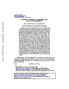
4. Empirical Likelihood control chart The EL quality control chart for the population mean that it is proposed in this paper is based, as we have commented, in the method of non-parametric inference Empirical Likelihood. We can distinguish two phases in its construction, equivalent to Phases I and II in the Shewhart’s control chart. In Phase I we estimate the unique control limit, using Empirical Likelihood with Bootstrap resampling calibration that will allow, in general, to compute with enough accuracy this limit; in Phase II, it is calculated for each sample of observations −2log( R( X )) , value that will be compared with the control limit to decide if it can be accepted that the process is in-control. A detailed description of the construction of the chart follows (figure 1): [INSERT FIGURE 1 OVER HERE] Phase I: estimation of the control limit. •

A Bootstrap procedure is applied to the m ⋅ n observations, drawing with

replacement B random samples of size n from the observed one. •

For each Bootstrap samples, C *b = −2 log( R *b ( X )) is calculated; so the

order set C (1) ≤ C (2) ≤ … ≤ C ( B ) is obtained. •

The unique control limit is computed as the percentile (1- α )% of the

previous values, using a Kernel smoother [Chou, Mason and Young (2001)] to find the α cutoff point, being α the desired probability of false alarm. Once the control limit and the rejection region of the chart are found, we can proceed to Phase II. Phase II:

For each new sample of size n the R( X ) value is calculated and −2 log( R( X )) is plotted in the chart. If −2 log R( X ) > CL , it is rejected that the process is an in-control state.

8

5. Analysis of Performance In order to study the performance of the EL control chart, a comparison with the rest of the considered charts ( X of Shewhart, EWMA, WV and Bootstrap) is carried out trough a simulation experiment. The following cases have been considered:

I. Distributions of the variable: samples coming from distributions standard Normal, t of Student with 3 degrees of freedom and Gamma(1.5, 20) has been simulated. Also, some possible mixtures among populations has been considered through the distributions symmetrical bimodal [50% N(0,1) and 50% N(4,1)] and the distribution asymmetric bimodal [95% N(0,1) and 5% N(4, 1/3)].

These bimodal distributions are often used in biological and

chemical industry, Faddoul et al. (1996). In this way we take into account, besides the normal distribution, a symmetrical distribution not normal, an asymmetric distribution, and two bimodal distributions. The Figure 2 shows the utilized distributions.

[INSERT FIGURE 2 OVER HERE]

II. Amount of sample information in Phase I: we will use in a combined way m samples of size n, considering the values m ⋅ n = 20, 50, 100 and 300 . That is to say, we consider the case in which we only have 20 observations in the Phase I to obtain the control limit, up to 300 observations in Phase I. III. Sample sizes in Phase II: for this comparison the following values of sample size are employed: n = 3, 5 and 10. IV. In-control ARL: we consider the cases in-control ARL = 333.3 (α = 0.003) and in-control ARL = 200 (α = 0.005). In this article we present the tables of

9

results when in-control ARL = 200. The tables with the results for in-control ARL = 333.3 are available from the authors, where all the conclusions are very similar.

To obtain the control limit of the EL control chart B = 2000 Bootstrap samples of size n were employed applied to the m ⋅ n initial data. The Matlab® functions used to make the simulations are available from the authors upon request. Tables 1 to 4 show the incontrol ARLs obtained by simulation. The asterisked values are the closest to the theoretical value desired for a given case. For the four charts considered, these ARLs are the average of 100 simulated charts, having each one 10000 points obtained via simulation of Phase II, after computing the control limit(s) in Phase I. [INSERT TABLE 1 OVER HERE] [INSERT TABLE 2 OVER HERE] [INSERT TABLE 3 OVER HERE] [INSERT TABLE 4 OVER HERE] After considering Tables 1 to 4 the following conclusions can be obtained. In first place, Table 1 (the case of having only m ⋅ n = 20 data in Phase I) shows that all the charts considered have a poor performance. This is a logical consequence of having such a few information available in order to obtain a precise estimation of the control limit(s). However, the EL control chart shows a consistent better performance for the majority of the cases studied. The empirical in-control ARL values obtained for this chart ranges from 34.13 to 84.75. Although these results are unsatisfactory, in the majority of the cases they are better in comparison against the rest of charts. For example, the in-control ARL values of the Bootstrap chart ranges from 15.41 to 53.19, the WV chart varies from 14.24 to 227.78. The empirical in-control ARL for de EWMA chart obtains its smallest value, 2.38, when the distribution is symmetric bimodal and n = 10, and the maximum value is 62.39 when n = 3, for the same distribution. The X chart shows a good performance when the symmetric bimodal distribution is simulated for n = 3, having an in-control ARL equals to 147.06. In general, considering also Tables 2 to 4,

10

the X chart shows a good performance for this distribution, even better than with the Normal distribution. The X chart outperforms all the charts for the case of n = 3 and Normal distribution in all the Tables. The WV chart shows the closet ARL value to 200 when n = 5 and the symmetric bimodal distribution is employed. However, for the rest of cases, the EL control chart obtains the best approximations to the theoretical ARL value (12 of the 15 cases studied).

When more data are available in Phase I, m ⋅ n = 50 (Table 2) again the EL control chart is, in general, the chart that produces in-control ARL values closer to the theoretical ARL = 200 but, as we may expect, obtaining better performance than in the case m ⋅ n = 20. For the same cases cited before, the X chart outperforms the EL chart. Again the WV chart is the best option when n = 5 and the symmetric bimodal distribution is used. When sample sizes are n = 5 or n = 10 the EL chart performs better than when n = 3, independently of the distribution considered. The EL chart is the best option in 11 out of of the 15 cases considered.

The case m ⋅ n = 100 is considered in Table 3. The X chart shows again a better performance when the distribution considered is the symmetric bimodal, when the Phase II sample size is n = 3 , or the Normal distribution when n = 3. If the observations are obtained from a Gamma(1.5, 20) distribution, the EWMA control chart shows the closest in-control ARL value, ARL=197.33. In this Table, the WV charts is the best option when n = 10 and the data is distributed as a symmetric bimodal. For the rest of cases, the EL control chart clearly outperforms the other charts. It is necessary to comment the bad and very similar performance of X , WV, Bootstrap and EWMA charts for the case of the t3 distribution. These charts obtained always an empirical incontrol ARL values from 20 to 50 for all the cases, whilst the EL chart performs better. Again, the results for the EL control chart are better when n = 5 or n = 10. The EL chart is the best option in 11 out of the 15 cases considered in this Table.

11

Finally, in Table 4, the amount of data available in Phase I is quite large, m ⋅ n = 300. The EL chart is the best option in 11 out of the 15 cases considered, with in-control ARL values ranging from 144.93 to 181.82. Even in the case of normality the X control chart does not obtain the closest values to the desired ARL = 200, although the differences with the best alternatives are small. However, it is the best option when n = 10 and for the symmetric bimodal distribution. The WV chart is the best alternative when n = 5 and the G(1.5, 20) distribution is simulated, with an in-control ARL equals to 181.82. The EWMA chart shows the best performance for the t3 distribution when n = 3 and for the Normal distribution when n = 10. A special case is the behavior of the EWMA chart when the data come from a symmetric bimodal distribution. In all the cases studied (see all the Tables), this chart shows a poor performance, with very low in-control ARLs.

As a general conclusion, it seems that the EL control chart proposed on this paper is a quite reliable control procedure when the distribution of the variable is not known or it is not Normal, although a minimum amount of data (about m ⋅ n ≥ 100) is necessary in Phase I.

6. Performance for Shift Detection In this section the performance of the EL control chart is studied when there is a shift in the process mean during Phase II. In addition, the X , EWMA, Bootstrap and WV charts are included in this study. It is important to outline the problem that arises when comparing the effectiveness of several charts for detecting process shifts, like, in this case, the in-control ARL values are not the same for all of them. In principle, this comparison is only possible in the case of having all the charts the same in-control ARL values. If this does not happen, the comparison is not fair, because it is favored to those schemes that have lower in-control ARL values. Therefore, we could obtain as a result that a control chart is more efficient when detecting a process shift, but, in the reality, this situation is obtained as a consequence of not having obtained the desired in-control

12

ARL value, but a lower one, producing more false alarms when the process is incontrol. Despite of this problem, we have carried out this study for the following reasons. In first place, it should be kept in mind that the user of a chart applied to control an unknown distribution does not know the value of the ARL value, neither the effectiveness when detecting shifts. In this section, we show the performance of some charts in front of some well-known distributions. In second place, although the results shows that the EL control chart obtains empirical in-control ARL values closer to the required one, it is necessary to check that this chart has the ability of detecting process shifts.

Finally, by means of this study we want to show another of the present problems in the charts studied. It is the asymmetric performance with regard to the direction of the shift. For example, when the distribution is normally distributed, the effectiveness of the X Shewhart control chart is studied in function of the shift measure d = m1 − m0 / σ 0 , where m1 is the mean when the process is out-of-control. The results commonly are only shown for positive values of d. In this case, this approach is correct, as its effectiveness does not depend on the direction of the shift, that is to say, it is the same performance for m1 = m0 ± dσ 0 . However, when the distribution of the quality characteristic is not symmetrical, the study of the effectiveness of the chart depends on the direction of the shift.

Figure 3 shows a histogram with the values of X when simulating a quality control chart with data coming from a Gamma(1.5, 20), histogram obtained with 10000 samples of size n = 5 . In the same figure the control limits obtained in the usual way (3-sigma criteria) are shown. As it can be observed, as the original distribution is right skewed, the distribution of the sample mean values, with this sample size, it is also right skewed. The right tail of the distribution is practically the one that provides the empirical value of probability of the Type I error. As it is easy to check, the control chart detects with more probability increments in the mean of the variable (figure 4) than decrements. This

13

situation is reflected in the following tables, Tables 5 and 6, where positive and negative shifts are considered. [INSERT FIGURE 3 OVER HERE] [INSERT FIGURE 4 OVER HERE] [INSERT TABLE 5 OVER HERE] [INSERT TABLE 6 OVER HERE]

The results that are showed in the Tables 5 and 6 are for the case m ⋅ n = 300 observations in Phase I to calculate the control limit(s) and samples of size n = 3 and 10 are employed during Phase II. The desired in-control ARL is 200. Tables show the empirical in-control ARL value obtained from previous tables when d = 0 and the empirical ARL values when there is a shift d ≠ 0, where the new mean m1 is m1 =

m0 ± dσ 0 . In order to compute the ARL values the same procedure as in the in-control scenario was followed (average of 100 simulated charts, having each one 10000 points obtained via simulation of Phase II, after computing the control limit(s) in Phase I).

The following conclusions can be obtained from the tables. The X control chart, as outlined before, has a no symmetric performance for asymmetric distributions. This different performance is only important for small process shifts (d = 0.2 and 0.5). For example, Table 5, for the distribution Gamma(1.5, 20) we obtain a value of ARL equals to 43.86 for d = 0.2, and 121.95 for d = -0.2. Following the same case, a value of ARL equals to 21.23 for d = 0.5, and 117.64 for d = -0.5 are obtained. When the sample size increases, Table 6, this difference tends to be smaller. Again with the distribution Gamma(1.5, 20), we obtain ARL = 8.43 for d = 0.5 and ARL = 9.82 when d = -0.5. For symmetric distributions, as we expected, the performance is equivalent. Due to the procedure followed to compute the control limits, the WV control chart obtains a similar performance in comparison with the X chart. On the other hand, the Bootstrap control chart has also similar behavior, not having symmetric behavior for the asymmetric distributions. The performance of the EWMA control chart is similar to the other charts

14

considered. This chart does not show a symmetric behavior for the asymmetric distributions, although the differences in the ARL values are less important when d increases. For example, for n = 3 and Gamma(1.5, 20) distribution, ARL(d = 0.2) = 51.92 and ARL(d = -0.2) = 23.73. However, ARL(d = 1.5) = 2.84 and ARL(d = -1.5) = 2.96 are very similar values. Now, if we consider the asymmetric bimodal distribution, for the same sample size, we obtain that ARL(d = 0.5) = 18.32 and ARL(d = -0.5) = 7.25, showing again the asymmetric performance of this chart.

For symmetric distributions the EL control chart shows a symmetric performance. For example, from Table 5, t3 distribution, ARL(d = 0.5) = 82.64, and ARL(d = -0.5) = 85.47. As it is expected, this chart increases its performance to detect shifts as the shift magnitude and/or the sample size increases. For example, following with the t3 case, the ARL(d = 1) = 29.50 for n = 3 and ARL(d = 1) = 4.08 for n = 10. Although the incontrol ARL values are not the same for the cases n = 3 and n = 10, as the in-control ARL value for n = 3 is smaller, it is possible to conclude that the performance is better when the sample size increases. For the asymmetric distributions studied, Gamma(1.5, 20) and asymmetric bimodal, the EL control chart also shows an asymmetric performance. As occurs with the rest of charts, this problem is less important for the case n = 10. For n = 10 and in the case of the asymmetric bimodal distribution, the difference is only important for small shifts.

As we commented above, it is not possible to make a performance comparison among the charts to detect process shifts, if they do not have the same probability of false alarm. However, the reader can check the global performance of the charts studied here in function of the different distributions studied. Nevertheless, it is very important to check that the EL control chart defined in this paper has the ability of detecting process shifts, i. e., it shows lower ARLs when the magnitude of the process shift increases, and it can detect large process shifts employing few samples. Considering Tables 5 and 6, it is possible to check that the EL control chart can detect large process shifts quickly, even in the cases when the in-control ARL is close to the required value of 200. For

15

example, for the Normal distribution, the out-of-control ARLs for a shift d = 2 are 4.56 for n = 3 and 1.00 for n = 10. In the case of the t3 distribution, the out-of-control values for d = -2 are 2.46 for n = 3, and 1.01 for n = 10.

In general, when the sample size is n = 10, the out-of-control ARLs are very close to the minimum value of 1. For the case of n = 3 the out-of-control values for d = 2 and -2 are of the same magnitude that the rest of charts, taking again into account that these values are not directly comparable. If we consider small process shifts (d = 0.2, 0.5 and -0.2, 0.5) clearly the EL control chart shows that it is able to detect these small shifts, obtaining significant lower ARL values in comparison with the in-control ARL. If the t3 distribution is taken as example, the in-control ARL for n = 10 is 175.44. Then, a very small process shift of size d = 0.2 is detected with an ARL equals to 55.25, and a shift of size d = 0.5 is detected with an ARL of 11.75. As a conclusion, the EL control chart can detect the out-of-control state of a process, with reasonably low values of ARL.

7. Example of Application To illustrate the use of the EL control chart for the process mean an example of application is showed in this section. Let us suppose that a mean of a quality characteristic has to be controlled employing a sample size n = 5. For this purpose, following the habitual procedure, 20 samples (m = 20) each one with a sample size of 5 (n = 5), have been collected during the Phase I when the process is considered to be in an in-control state, that is to say, m ⋅ n = 100. The 100 obtained values used in this application example and the Matlab® functions employed are available from the authors.

The distribution of the population of this variable is ignored. But the conclusions obtained in this article suggest that with m ⋅ n = 100 values obtained in Phase I, the EL control chart will provide a control procedure where the empirical and the desired in-

16

control ARL values will be very similar, obtaining, also, a reasonable performance for the detection of process shifts.

The sample mean of the m ⋅ n = 100 data is 29.3597, value that will be used for the EL test as in-control mean. Applying the procedure developed in this paper we obtain that the control limit is 14.1927. Finished the Phase I, we could begin to the control the process using the EL control chart. Table 7 shows the obtained samples during the Phase II, and the value of the statistical EL to plot associated to each sample. As we can see, the last sample overcomes the control limit and, therefore, we would reject that the process is in-control.

[INSERT TABLE 7 OVER HERE]

CONCLUSIONS In this paper we proposed a control chart for the process mean based on Empirical Likelihood. The results of the simulations carried out show that the EL provides, in most of the studied conditions, robust values of in-control ARL, close to the required one, regardless the distribution of the utilized data, and sample sizes considered in the Phase II of the process. For obtaining this good performance it seems not necessary to have a large amount of data available in Phase I. In addition, the EL chart is able to detect the possible process shifts with a performance that seems reasonable.

Acknowledgements. The authors acknowledge the financial support of the Ministry of Education and Science of Spain, Research Project Reference DPI2006-06124 and European FEDER funding.

17

REFERENCES.

Alloway, J. A.; and Raghavachari, M. Control Chart Based on the Hodges-Lehman Estimator. Journal of Quality Technology 1991 23; pp. 336-347. Aparisi, F and García-Díaz, J. C. Optimization of Univariate and Multivariate Exponentially Weighted Moving Average Control Charts using Genetic Algorithms. Computers and Operations Research, 2003, 31(9), 1437-1454. Bai, D. S.; and Choi, I. S.. X and R Control Charts for Skewed Populations. Journal of Quality Technology 1995 27; pp. 120-131. Bajgier, S. M. The use of Bootstrapping to Constructs Limits on Control Charts. Proceedings of the Decision Science Institute, San Diego, CA, 1992; pp. 1611-1613. Chakraborti, S., Van Der Laan, P. and Bakir, S. T. Nonparametric Control Charts: An Overview and Some Results. Journal of Quality Technology 2001 33; pp. 304-315. Chou, Y.; Mason, R. L.; and Young, J. C. The Control Chart for Individual Observations from a Multivariate Non-Normal Distribution. Communications on Statistics. Theory & Methods 8&9 2001; pp. 1937-1949. Davison, A. C.; and D. V. Hinkley. Bootstrap Methods and their Application, Cambridge, Cambridge University Press, 1997. Devor, R. E.; Chang, T.; and Sutherland, J. W. Statistical Quality Design and Control. Macmillan, NY, 1992. Efron, B. Bootstrap Methods: Another Look at the Jackknife. Annals of Statistics 1979 7; pp. 126. Efron, B. The Jacknife, the Bootstrap and other Resampling Plans. Society for Industrial and Applied Mathemathics, Philadelphia, PA, 1992. Efron, B. Better Bootstrap Confidence Intervals. Journal of the American Statistical Association 1987 82; pp. 171-175. Efron, B. More Efficient Bootstrap Computations. Journal of the American Statistical Association 1990 85; pp. 79-89. Efron, B. and Tibshirani, R. J. An Introduction to the Bootstrap, Chapman & Hall, 1993. Faddoul, N. R., English, J. R. and Taylor, G. D. The Impact of Mixture Distributions in Classical Process Capability Analysis. IEE Transactions 1996 28; pp. 957-966. Ferrell, E. B. Control Charts for Lognormal Universe. Industrial Quality Control 1958 15; pp. 4-6. Jones, L. A.; and Woodall, W. H. The Perfomance of Bootstrap Control Charts. Journal of Quality Technology 1998 30, No 4; pp. 362-375.

18

Kittlitz, R. G. Jr. Transforming the Exponential for SPC Applications. Journal of Quality Technology 1999 31; pp. 301-308. Leger, C.; Politis, D.; and Romano, J. Bootstrap Technology Applications. Technometrics 1992 34; pp. 378-398. Lehmann, E. L. Nonparametric Confidence Intervals for a Shift Parameter. The Annals of Mathematical Statistics 1963 34; pp. 1507-1512. Liu, R. Y.; and Tang, J. Control Chart for Dependent and Independent Measurements Based on Bootstrap Methods. Journal of the American Statistical Association 1996 91; pp. 1694-1700 Montgomery, D. C. Introduction to Statistical Quality Control. 4rd edition, Wiley, New York, 2001. Nelson, R. P. Control Charts for Weibull Processes with Standards Given. IEEE Transactions on Reliability 1979 28; pp. 283-298. Owen, A. B. Empirical likelihood confidence intervals for a single functional. Biometrika 1988 75; pp. 237-249. Owen, A. B. Empirical likelihood confidence regions. The Annals of Statistics 1990 18; pp. 90120. Owen, A. B. Empirical Likelihood. Chapman & Hall, London, 2001. Hunter JS. The exponentially weighted moving average. Journal of Quality Technology 1986; 18: 155-162. Pappanastos, E. A. and Adams, B. M. Alternative Designs of the Hodges-Lehman Control Chart. Journal of Quality Technology 1996 28; pp. 213-223. Seppala, T.; Moskowitz, H.; Plante, R.; and Tang, J. Statistical Process Control via the Subgroup Bootstrap. Journal of Quality Technology 1995 27; pp. 139-153. Shewhart. W. A. Statistical Methods from the Viewpoint of Quality Control, 1931. Republished in 1986 by Dover Publications. Schilling, E. G.; and Nelson, P. R. The effect of Non Normality on the Control Limits of X Charts. Journal of Quality Technology, 1976 Vol 8, No 4; pp. 183-188. Vermat, M. B.; Ion, R.; Does, R.J.; and Klaassen, C. A Comparison of Shewhart Individuals Control Chart Based on Normal, Non-Normal, and Extreme Value Theory. Quality and Reliability Engineering International 2003 19; pp. 337-353. Willeman, T. R. and Runger, G. C. Designing Control Charts Using an Empirical Reference Distribution. Journal of Quality Technology 1996 28; pp. 31-38. Wilks, S. S. The large-sample distribution of the likelihood ratio for testing composite hypotheses. Ann. Math. Stat. 1938 9; pp. 60-62.

19

FIGURE 1

Figure 1. Empirical Likelihood control chart, showing phases I and II.

20

FIGURE 2

Normal (0, 1)

Symmetric Bimodal

Gamma (1.5, 20)

Asymmetric Bimodal

t3

Figure 2. Probability density of the variables employed.

21

X

Bootstrap

EL

WV

EWMA

n

3

5

10

3

5

10

3

5

10

3

5

10

3

5

10

t3

25.25

22.47

17.30

16.81

15.41

18.28

34.13*

47.62*

41.32*

22.99

21.01

14.25

11.44

11.62

5.23

Normal

59.17*

48.31

34.01

31.35

32.47

24.63

34.01

60.24*

84.75*

54.95

43.29

32.79

14.59

8.98

8.76

G(1.5,20)

30.67

24.51

20.62

28.90

19.19

19.46

40.32*

50.00*

51.02*

38.61

28.25

22.27

62.39

22.21

9.24

147.06*

62.50

26.95

53.19

51.28

25.38

34.84

52.63

71.94*

277.78

96.15*

40.16

5.04

4.34

2.38

29.59

25.77

24.33

22.12

19.61

18.90

34.25*

65.36*

62.50*

29.85

24.10

22.78

14.13

11.12

5.36

Symmetric bimodal Asymmetric bimodal

Table 1. In-control ARL values for the case m·n = 20 observations in Phase I. Phase II sample size n = 3, 5, 10. The asterisk (*) indicates the closest value to the desired ARL(d = 0) = 200.

22

Bootstrap

X

EL

n

3

5

10

3

5

10

t3

35.46

37.17

32.15

32.26

31.75

27.55

Normal

108.70*

80.65

76.92

71.43

72.99

G(1.5,20)

44.05

38.61

52.36

56.18

312.50*

142.86

89.29

56.82

73.53

55.56

Symmetric bimodal Asymmetric bimodal

3

5

WV 10

EWMA

3

5

10

3

5

10

70.92* 113.64* 114.94*

33.44

34.60

30.40

31.27

16.24

9.53

62.50

94.34

104.17

80.65

73.53

36.92

18.05

13.07

51.02

56.50

76.92*

93.46

105.26*

59.17

49.50

65.36

45.76

125.45*

11.17

74.63

99.01

78.13

78.13

104.17

131.58*

454.55 200.17* 113.64

4.79

4.15

2.16

61.35

75.76

50.51

68.97* 109.89* 103.09*

60.24

23.33

21.97

9.77

129.87* 117.65*

77.52

50.25

Table 2. In-control ARL values for the case m·n = 50 observations in Phase I. Phase II sample size n = 3, 5, 10. The asterisk (*) indicates the closest value to the desired ARL(d = 0) = 200.

23

Bootstrap

X

EL

n

3

5

10

3

5

10

t3

43.29

47.17

50.00

47.17

46.73

42.92

Normal

144.93*

133.33

111.24

119.05

106.38

G(1.5,20)

58.82

70.42

69.93

92.59

588.24

243.90*

158.73

78.13

87.72

102.04

Symmetric bimodal Asymmetric bimodal

3

5

WV 10

EWMA

3

5

10

3

5

10

103.09* 142.86* 144.93*

41.67

45.66

45.66

35.30

32.88

17.39

104.17

112.36

147.06* 142.86*

140.85

129.87

105.26

39.34

24.75

19.94

95.24

88.50

103.09

140.85* 151.52*

82.64

102.04

98.04

197.33*

51.71

17.05

120.48

127.71

128.21

129.61*

153.85

155.32

909.09

312.50

188.68*

4.80

3.94

2.56

109.89

112.36

98.04

119.27* 154.27* 119.05*

87.72

96.15

99.01

31.93

20.54

18.28

Table 3. In-control ARL values for the case m·n = 100 observations in Phase I. Phase II sample size n = 3, 5, 10. The asterisk (*) indicates the closest value to the desired ARL(d = 0) = 200.

24

Bootstrap

X

EL

n

3

5

10

3

5

10

3

t3

55.56

55.87

62.11

81.97

78.74

69.93

144.93

Normal

178.41

178.57

158.73

156.25

161.29

140.85

181.82*

G(1.5,20)

69.93

81.97

101.01

149.17

149.25

1000.00

370.37

204.08*

151.52

95.24

120.48

120.48

142.86

Symmetric bimodal Asymmetric bimodal

5

WV 10

EWMA

3

5

10

3

5

10

169.49* 175.44*

54.95

55.25

60.98

158.40*

296.07

253.63

169.37

169.49

177.84

181.82*

156.25

107.35

58.83

205.27*

138.89

163.93* 161.29* 172.41*

105.26

129.87

151.52

150.14

130.03

148.03

171.44

138.22

175.67* 172.41*

176.31

1111.19

400.07

222.32

5.14

3.96

2.34

151.52

144.93

166.67* 172.92* 175.34*

108.70

140.85

136.99

52.09

34.80

21.13

Table 4. In-control ARL values for the case m·n = 300 observations in Phase I. Phase II sample size n = 3, 5, 10. The asterisk (*) indicates the closest value to the desired ARL(d = 0) = 200.

25

d (shift in sigma units) 0

0.2

0.5

1

1.5

2

X

chart

-0.2

-0.5

-1

-1.5

-2

t3

55.56

43.86

25.19

6.34

2.03

1.22

44.84

25.77

6.45

2.02

1.21

Normal

178.41

111.11 33.90

6.65

2.33

1.97

117.65

36.23

6.90

2.38

1.34

G(1.5,20)

69.93

43.86

6.99 27.47 1.41

121.95 117.64

8.47

2.14

1.31

Simetric bimodal Assimetric bimodal

21.23

1000.00 769.23 243.90 51.81 17.76 8.75 95.24

71.43

40.82 15.27 5.98

2.64

909.09 285.71 56.82 18.98 10.75 116.28

88.50

19.53

4.96

2.12

BOOTSTRAP t3

81.97

73.53

45.87 12.48 3.61

1.79

67.11

15.13

9.89

3.01

1.59

Normal

156.25

97.09

30.96

1.84

104.17

33.22

6.65

2.36

1.34

G(1.5,20)

149.25

153.85 70.42 21.23 71.43 2.90

26.67

5.51

1.83

1.23

1.07

Simetric bimodal Assimetric bimodal

151.52

121.95 57.47 19.31 9.24 51.81 126.58

60.61

20.12

9.54

5.32

142.86

188.68 136.99 51.55 17.54 6.26

97.09

33.78

7.22

2.64

1.54

6.38

2.30

EL t3

144.93

126.58 82.64 29.50 7.57

2.45

129.87

85.47

30.77

7.78

2.46

Normal

181.82

142.86 89.29 23.64 6.10

4.56

140.85

89.21

24.88

6.28

2.37

G(1.5,20)

163.93

112.36 58.82 17.61 7.50

3.00

175.44 165.18 107.53 9.12

2.45

Simetric bimodal Assimetric bimodal

175.67

144.93 100.00 41.67 18.98 10.00 149.25 103.09 44.05 19.49 10.32

166.67

166.67 129.87 70.42 31.95 11.93 188.68 185.19 138.89 44.84 10.18 WV

t3

54.95

43.67

2.04

1.23

43.86

24.94

6.24

1.99

1.21

Normal

177.84

112.36 34.25 67.11 2.34

1.99

114.94

35.34

6.80

2.37

1.34

G(1.5,20)

105.26

65.79

1.70

185.19

69.23

4.20

1.66

1.19

Simetric bimodal Assimetric bimodal

25.25

31.45

6.37

9.93

3.67

1111.19 909.09 270.27 54.05 18.15 8.86 1000.00 303.03 56.82 18.87 9.11 108.70

89.29

51.55 19.19 7.29

3.09

119.05

68.03

13.70

3.90

1.86

EWMA t3

158.40

30.90

9.50

4.10

2.76

2.15

35.35

9.83

4.03

2.83

2.12

Normal

107.35

26.62

20.10

4.28

3.07

2.24

2.56

11.05

4.82

2.78

2.27

G(1.5,20)

150.14

51.92

9.43

4.85

2.84

2.24

23.73

8.32

4.71

2.96

2.20

Simetric bimodal Assimetric bimodal

5.14

6.69

14.20 55.24 8.02

4.09

4.03

3.21

2.33

1.99

1.73

52.09

84.07

18.32

2.40

14.12

7.25

3.81

2.65

2.12

5.25

3.19

Table 5. ARL values for m·n = 300 observations in Phase I, Phase II sample size n = 3, and required ARL(d = 0) = 200

26

d (shift in sigma units) 0

0.2

0.5

1

1.5

X

2

-0.2

-0.5

-1

-1.5

-2

chart

t3

62.11

36.63

7.92

1.44

1.05 1.00

37.04

7.99

1.46

1.03 1.00

Normal

158.73

60.24

8.84

1.59

1.03 1.00

59.17

8.70

1.58

1.03 1.00

G(1.5,20)

101.01

36.23

8.43

1.67

1.02 1.00

147.06

9.82

1.50

1.04 1.00

Simetric bimodal

204.08

142.86

50.25

11.25

3.90 1.95

151.52

54.64

11.93

4.06 2.01

Assimetric bimodal

120.48

66.67

19.23

3.53

1.34 1.02

126.58

21.55

2.87

1.35 1.09

BOOTSTRAP t3

69.93

45.87

10.26

1.77

1.08 1.01

42.37

9.47

1.75

1.09 1.01

Normal

140.85

49.75

7.96

1.55

1.03 1.00

55.25

8.47

1.58

1.03 1.00

G(1.5,20)

138.89

78.13

16.37

2.47

1.08 1.00

25.64

3.65

1.21

1.01 1.00

Simetric bimodal

138.22

106.38

39.22

9.35

3.45 1.81

117.65

44.25

10.31

3.68 1.89

Assimetric bimodal

144.93

125.00

35.97

5.56

1.67 1.07

59.17

10.72

2.16

1.23 1.08

EL t3

175.44

55.25

11.75

4.08

1.60 1.14

59.52

12.06

4.12

1.67 1.14

Normal

169.49

88.50

20.04

3.85

1.52 2.85

85.47

19.61

3.80

1.52 1.07

G(1.5,20)

172.41

322.58

52.91

2.54

2.73 1.22

66.67

25.45

8.37

2.62 1.44

Simetric bimodal

176.31

136.99

69.93

18.66

5.73 2.38

142.86

72.99

19.38

5.95 2.45

Assimetric bimodal

175.34

192.31

48.78

8.31

3.42 1.87

69.93

22.52

8.12

4.42 2.00

WV t3

60.98

35.84

7.82

1.45

1.04 1.00

35.59

7.75

1.46

1.03 1.00

Normal

156.25

58.82

8.76

1.59

1.03 1.00

58.48

8.67

1.58

1.03 1.00

G(1.5,20)

151.52

58.14

12.45

2.06

1.04 1.00

56.50

5.33

1.31

1.02 1.00

Simetric bimodal

222.32

158.73

53.76

11.66

3.96 1.96

163.93

56.18

12.05

4.05 1.99

Assimetric bimodal

136.99

86.21

24.45

4.17

1.45 1.04

90.09

15.20

2.47

1.28 1.06

EWMA t3

253.63

14.24

3.96

2.00

1.32 1.05

14.89

4.54

1.96

1.27 1.03

Normal

205.27

24.63

3.80

2.20

1.38 1.05

19.18

4.23

2.19

1.39 1.06

G(1.5,20)

148.03

8.59

4.58

2.07

1.38 1.04

17.90

5.21

2.04

1.36 1.08

Simetric bimodal

2.34

2.97

6.52

21.30

3.55 1.93

1.92

1.50

2.07

1.00 1.00

Assimetric bimodal

21.13

46.81

6.68

2.44

1.61 1.11

7.01

3.20

1.85

1.21 1.02

Table 6. ARL values for m·n = 300 observations in Phase I, Phase II sample size n = 10, and required ARL(d=0) = 200

27

Figure 3. Distribution of 10000 values of X when n = 5 and the distribution is a

Gamma(1.5, 20). Shewhart control limits are showed.

Figure 4. Same distribution as figure 3 when a positive shift in the mean occurs.

28

Sample

Data

EL statistic

1

4.4288 11. 3808 24. 3718 26. 2568 17. 2304

1. 5562

2

74. 2509 9. 6053 18. 9874 32. 8595 17. 5490

0. 0164

3

9. 7315 45. 7000 9. 2347 77. 1196 3. 579

0. 0005

4

50. 9460 7. 5027 70. 6616 51. 1312 38. 8743

2. 0152

5

13. 7145 1. 0721 61. 0591 6. 9067 20. 9179

0. 6604

6

4. 7270 67. 2110 3. 5845 5. 0557 26. 3864

0. 4421

7

13. 5978 13. 7097 28. 4883 16. 8079 16. 1233

1. 3168

8

10. 6024 33. 7062 36. 3889 43. 1536 65. 1888

1. 1438

9

23. 3527 46. 1669 2. 0657 3. 7675 58. 5665

0. 0646

10

69. 8863 58. 7792 66. 2198 87. 6878 43. 7330

14. 974 > CL

Table 7. Samples and associated EL statistics for the example of application.

29