Department of Computer Science, Univ. of Massachusetts, Amherst. {nilanb ... If the nodes are too liberal with their energy consumption, they will fail pre- maturely. .... or they are built assuming very specific movement patterns of nodes [20].
1
An Energy-Efficient Architecture for DTN Throwboxes Nilanjan Banerjee Mark D. Corner Brian Neil Levine Department of Computer Science, Univ. of Massachusetts, Amherst {nilanb,mcorner,brian}@cs.umass.edu
I. I NTRODUCTION Recent efforts in Disruption Tolerant Networking (DTN) promise networking infrastructures that are robust to widespread failures and operate in highly challenged environments [7, 9, 2]. Such networks can be used to route information in completely unconnected and decentralized scenarios, including natural disasters, sparse sensor deployments, underwater networking, and highly mobile systems. DTNs rely on intermittent contacts between mobile nodes to deliver packets using a store-carry-and-forward paradigm. The routing performance in a DTN, including deliverability and delay, is critically dependent on the node mobility patterns that drive the frequency, duration, and sequence of contact opportunities. One method to improve these metrics is to engineer a greater number of opportunities. For instance, several papers have proposed altering the mobility of nodes to enhance network performance [3, 4, 26, 8]. Unfortunately, movement patterns are often inherent to the nodes and cannot be modified. Another solution for improving DTN performance is to place additional stationary nodes in the network, which increases the number and frequency of contact opportunities. In previous work, we proposed the use of throwboxes within a DTN for this purpose [27]. Throwboxes are inexpensive, battery-powered, stationary nodes with radios and storage. When two nodes pass by the same location at different times, the throwbox acts as a router, creating a new contact opportunity. In our previous work, we focused on algorithms that place throwboxes in loca-
Contact opportunity
Speed and direction beacon
Throwbox
Mobile Node
Tier-0 Mote Xtend Radio
XTend Radio Range
802.11 Range
Mobility Prediction Lifetime Scheduler
Wa keu p
Abstract— Disruption Tolerant Networks rely on intermittent contacts between mobile nodes to deliver packets using store-carry-and-forward paradigm. The key to improving performance in DTNs is to engineer a greater number of transfer opportunities. We earlier proposed the use of throwbox nodes, which are stationary, battery powered nodes with storage and processing, to enhance the capacity of DTNs. However, the use of throwboxes without efficient power management is minimally effective. If the nodes are too liberal with their energy consumption, they will fail prematurely. However if they are too conservative, they may miss important transfer opportunities, hence increasing lifetime without improving performance. In this paper, we present a hardware and software architecture for energy efficient throwboxes in DTNs. We propose a hardware platform that uses a multi-tiered, multi-radio, scalable, solar powered platform. The throwbox employs an approximate heuristic for solving the NP-Hard problem of meeting an average power constraint while maximizing the number of bytes transfered by the throwbox. We built and deployed prototype throwboxes in UMassDieselNet – a 40 bus DTN testbed. Through extensive trace-driven simulations and prototype deployment we show that a single throwbox with a 270 cm2 solar panel can run perpetually while improving packet delivery by 37% and reducing message delivery latency by at least 10% in the network.
Tier-1 Stargate 802.11 Radio Routing Engine Packet Storage
Fig. 1. Overview of our throwbox architecture.
tions that maximize network performance. We found that even a small number of throwboxes can significantly increase the delivery rate found in a DTN. However, this addressed only part of the problem. Throwbox deployment without the use of power management is minimally effective. The high power consumption of alwayson nodes results in a short lifetime; conversely, nodes powering on and off intermittently without regard to node mobility may miss numerous connection opportunities, increasing lifetime without necessarily improving performance. The key goal is to provide energy efficiency without sacrificing network performance. Moreover, throwboxes are constrained to consume power at a rate dictated by a battery lifetime requirement or the availability of scavenged energy, such as solar power. In this paper, we address these issues in the context of the following challenge: how can a throwbox in a DTN meet an average power constraint and simultaneously maximize the number of packets delivered? We show that the primary source of overhead is the energy cost of neighbor discovery: idling or turning the platform and radio on and off to search for contacts in a sparse network wastes the vast majority of node energy. Due to the sparseness of a DTN, waking up for non-existent, or brief, contact opportunities is not worth the cost of turning on the platform and radio. In this paper, we propose a novel paradigm for power management in DTNs that provides more efficient neighbor discovery by detecting the mobility of other nodes at a minimum cost and predicting the cost and opportunity of each possible contact. Using these predictions, the throwbox can intelligently choose the most fruitful contact opportunities, and it can limit the number of opportunities to meet energy constraints. In our architecture, we pair a tier-1 platform — a PDA-like Stargate and 802.11 radio — with a low-power tier-0 platform — a Mote and XTend radio. The XTend radio is a long-range, low-bitrate radio for
2
neighbor and mobility discovery. It has a range of more than a kilometer, which is more than five times the range of WiFi radios. By coupling the XTend radio with a low-power Mote, we reduce the total energy cost of the throwbox platform. Figure 1 presents an overview of our approach and the problems we address in this paper. Mobile nodes (shown as a bus in the diagram) beacon their position, direction, and speed using the long-distance radio. While listening for other nodes, the throwbox needs very little computational power and memory, and the tier-0 platform is sufficient to process the beacons. If a throwbox hears a beacon, tier-0 predicts if, when, and for how long the mobile node will come in contact with the tier-1, 802.11 radio. Using a constrained single-objective optimization to meet a power consumption target, the node decides whether to take the transfer opportunity. If it does, tier-0 wakes the Stargate and WiFi radio in advance of the mobile node entering radio range, which then transfers DTN data. After the contact opportunity, the tier-1 platform returns to a sleep state. For this scenario, we develop a method for predicting the contact opportunities based on the observed mobility of remote nodes and an algorithm for choosing which contacts to take given power constraints. We meet our objectives through a mix of theoretical and practical results. In Section III, we present a mobility prediction algorithm that is sufficiently lightweight to operate on a Mote. Section IV presents a duty-cycling algorithm for the long range radio. In Section V, we detail our scheduling algorithms that help meet an average power constraint for the throwbox while maximizing the number of packets delivered in the network. We present theoretical bounds on the complexity of the optimization problem and the performance of an online algorithm based on token-buckets. We show the problem is NP-Hard and present competitive bounds on the performance of the algorithms for a simple node mobility pattern. In Section VI, we detail our design and implementation of a prototype throwbox and its deployment and integration into the UMassDieselNet DTN [2]. And finally, we show the performance of the system through an extensive set of trace-driven simulations and experiments on the deployed platform. Our methods reduce the power consumption of the throwbox from 2500 mW to 80 mW while delivering almost as many packets. Stated another way, we have deployed a throwbox that runs perpetually on solar cells similar to the size of the box itself. II. BACKGROUND Peers in a mobile network alternate between two basic operations: neighbor discovery and opportunistically transferring data. In DTNs the latter operation has received much attention as part of routing protocols [2, 7]. However, in a sparse DTN network, searching for other nodes consumes a large percentage of time in comparison to transferring data. Consequently, searching for other nodes becomes the dominant drain on the energy of a battery-powered DTN node. For instance, we show in this paper that using an 802.11 radio to search for contacts in a DTN devotes 99.5% of the total energy just to find other nodes to exchange data with. Simple power management schemes are insufficient—a radio in idle mode has little savings as compared to its listening mode. Previous work has addressed mobile system power man-
agement by using 802.11 radios for data transfers and lowpower, short-range radios (e.g., 802.15.4 [14], Bluetooth [15], or CC1000 [16]) for neighbor discovery tasks. While this solution is appropriate for dense mobile networks, our recent work has shown it is inefficient for sparsely populated DTNs [11]— we strengthen this claim in this paper. This is because shortrange radios miss too many connection opportunities, which tend to be short-lived compared to the delay and cost of switching 802.11 radios from sleep to wake modes. Moreover, these architectures do not reduce the cost of other idle hardware components, predict the mobility of the node, nor choose which opportunities to take. A key to realizing the gains of a second radio is to be able to predict neighbor mobility before the node is within contact of the throwbox. Mobility prediction algorithms in the past have been used to predict future network topology to perform route reconstruction proactively [23], accurately predicting hand-offs and bandwidth provisioning in cellular networks [5, 20], and location tracking in wireless ATM networks [13]. Such algorithms either require coordinated information from more than one base station [20, 21], they are computationally too expensive to implement on a extremely low power tier-0 subsystem [21], or they are built assuming very specific movement patterns of nodes [20]. Most mobility predictors are assumed to be implemented on powerful base stations, which are unconstrained platforms. Mobility prediction has also been used in DTNs, taking advantage of a known schedule for mobile nodes in the network [12]. In our work, we develop prediction algorithms that are lightweight enough to run on a small, extremely efficient platform, such as a Mote. This helps minimize the cost for deciding which contact opportunities to take. Additionally our technique does not depend on any centralized infrastructure, or scheduled node mobility. III. M OBILITY P REDICTION E NGINE Because DTNs are sparsely populated, throwboxes must expend significant energy searching for contact opportunities. Because of node mobility, throwboxes have a limited amount of time to exchange data with peers. Searching for contacts efficiently requires waking and sleeping rapidly (called duty cycling), and conversely, data transfer requires high-bandwidth connections. Our design philosophy is to separate neighbor discovery from data transfer, and to divide these tasks across the hardware that is best suited to each task. The long-distance radio and tier-0 platform can duty-cycle, listen, and idle efficiently, while the high-bandwidth radio and tier-1 platform can transfer large amounts of data during limited connection opportunities. While the tier-0 platform is listening for contacts, the tier-1 platform remains asleep. The decision to wake the tier-1 platform and radio depends on an engine that detects, and predicts the mobility of nodes in the network, based on information gathered by the tier-0 platform and radio. By predicting the trajectory of an on-coming mobile node, the tier-0 platform can determine if, when, and for how long it will enter the range of the data transfer radio. If the throwbox determines that the mobile node will not come in contact with its data transfer radio, it can safely ignore that node. If it determines that the mobile node will enter at a certain time, it
3
D1 D2 A
Probability of entering 802.11 range from Cell A Traveling in the SE Direction P AB * P BC
B Predicted Time Before Node enters the 802.11 range D1 / Velocity
C 802.11 Range
Predicted Time Till Node Will remain in 802.11 Range D2 / Velocity
NODE TRAJECTORY
Fig. 2. The figure depicts the working of the Mobility Prediction Engine
must make sure that the throwbox can make the most out of the contact opportunity. When the throwbox estimates the time that the mobile node will enter 802.11 range, it wakes the tier-1 node in advance of the mobile node arriving—a process that can take several seconds. The predicted length of the contact opportunity is then used to determine which contact opportunities to take, a process we explain in Section V. To determine trajectories, we require that mobile nodes periodically transmit location, speed, and direction over the longdistance radio as a beaconing message. By requiring mobile nodes to beacon their positions, we have shifted some of the energy burden from the stationary throwboxes to the mobile nodes. In this paper, we study the use of throwboxes in a vehicular network, where the mobile nodes have plentiful energy sources. Nonetheless, the techniques will aid systems where all nodes are energy constrained as it lowers the cost of discovery; however, we leave this as future work. A. Prediction Algorithm We model the movement pattern of the mobile nodes as a Markovian process. Hence, we assume the location of a node at time Ti is dependent only on its location at time Ti−1 . Such a model is accurate for movement patterns that are both predictable and semi-predictable. The algorithm models the problem as a virtual square of width 2r, where r is the radius of the long-range radio. The throwbox is located at the center of the square, as illustrated in Figure 2. The large square is divided into square cells numbered from 0 to k. The algorithm makes use of a probability transition matrix T for mobile nodes in the network. Entry Tij of the matrix is the probability that a node will transition to cell j given that it is in cell i. Mobile nodes beacon data in tuples in the form < p, v, t, d >, where p is the present GPS location of the mobile node, v is its speed, t is the time at which the data was sent, and d is the direction of motion of the node. When a node n approaches, the throwboxes collect a set of tuples {< p1 , v1 , t1 , d1 >, ..., < pk , vk , tk , dk >}. Using this set, as well as historic information, the algorithm estimates : • The probability that the mobile node n would be in any cell within the data transfer radio range after time ∆T , where ∆T is the time required to wakeup tier-1 and start transferring ap-
plication data—it is typically on the order of seconds • The predicted time when the node will be in range of the data transfer radio and, subsequently, the amount of data it is likely to transfer Figure 2 illustrates this process. At time t = 0, the mobile node’s beacon from cell A is received. By dead-reckoning along a straight line of motion, the prediction engine estimates D1 , the distance until the node is within 802.11 range, and D2 , the distance for which the node would be within range, Accordingly, the predicted length of time until the mobile node reaches the range of the data radio is D1 /v; if this time is greater than the transition time to wakeup tier-1, then the mobile node is ignored. Otherwise, the throwbox calculates P r, the probability that the node will enter the range of the data radio. (In the simple example presented in the figure, P r is the product of the probability of transition from cell A to B and from B to C; i.e., P r = TAB · TBC .) The expected duration of time the mobile node will stay in data radio range is P r · (D2 /v). Below we show how we calculate P r under Markovian assumptions. B. Estimating the Probability of Entering Data Radio Range The prediction engine assumes that the node would move in the direction that it was last seen. Therefore, it constructs a straight line in the current direction of motion and finds the intersection with the range of the data-transfer radio range (idealized as a circle). Let p be the cell at which the node enters the data radio range; let Dp,pk be the Euclidean distance between the present location of the node and the location of the point where it enters the data transfer radio range (assuming the present direction of motion of the node); let vk be the velocity of node n; and let ci , . . . , cj+i be a sequence of cells that are in the predicted path of motion of the node. Let {d1 , . . . , di } be the set of i possible directions of motion. For example, a direction could be north, south, east or west. The probability that a node enters the data transfer radio range at position p after time ∆T is given by P r[Xtk +∆T = p|(Xtk = pk , dtk = dk ), . . . , (X1 = p1 , dt1 = d1 )], (1) where Xt is the position of the node at time t. The above probability can be approximated as Pappr = P r[Xtk +∆T = p|Xtk = pk , dtk = dk ]
(2)
assuming that the node movement is modeled as a Markovian process. Pappr is evaluated by the algorithm as P r[Xtk +∆T = p|(Xtk = pk , dtk = dk )] = ( Dp,pk ≤ ∆T Tci ,ci+1 · . . . · Tci+j−1 ci+j , vk 0,
Dp,pk vk
> ∆T
(3)
Equation 3 shows that the probability of a node entering a cell of the data transfer radio after time ∆T is equal to the transition probability of the node from its present cell to cell ci+j if the node is traversing fast enough to cover the shortest distance between the two cells in time ∆T .
4
IV. D ISCOVERY R ADIO D UTY-C YCLE C ONTROLLER If multiple contacts are simultaneously discovered by the throwbox, it takes the size of the connection event as the sum of the predicted connection size of each contact. We also note that while searching for mobile nodes, the longdistance radio does not need to be constantly powered; it needs to only wake-up often enough to predict if, when, and for how long the mobile node will be within range of the data transfer radio. This is consistent with past approaches to lowering wireless power consumption such as PSM [1], which duty-cycle the radio to save energy. Our throwbox design uses a MaxStream XTend radio that supports several very efficient duty-cycling modes at the hardware and MAC layer. The MAC protocol built into the longrange radios is very similar to the B-MAC protocol built for CC1000 Mote radios [17]. The radios used in this work are built with k software configurable cyclic sleep modes {S1 , S2 , ..., Sk }. In sleep mode Sk , the radio wakes up every tk seconds for time τ (τ 1,the probability that the percentage of connection events discovered is more than k1 is bounded by e−Ω(n) , where n is the number of contact opportunities. Proof: The scenario for the proof is illustrated in Figure 6. We assume that the throwbox is located at the center of the circle and a node enters the range of the large range radio at point A. The probability that the node would enter the range of the 2·sin−1 ( r )
R low power radio is at most . We assume that the conπ nection events occur independently of each other and follow a
binomial distribution with parameters (n,
r 2·sin−1 ( R ) ). π δ 2 ·np − 3
By Cher-
noff’s bound, P [B(n, p) > (1 + δ)np] ≤ e . Therefore, 1 P [B(n, p) ≥ n/k] ≤ e−Ω(n) if 1 − 2p > 0. Replacing p by r 2·sin−1 ( R ) , π
yields the result in the proposition. Also note that the size of the connection event detected by the short range radio is at most half of the total size of the connection event. Corollary 1: If we use the Zigbee radio (range = 50 m) as the 802.11 radio (range = 300 m) k = 9. This implies that the combination of a Zigbee and a 802.11 radio 89 of the connection events would not be detected with a very high probability.
5
Lemma 2: If r ≥ 3R, and the long range radio is awake with a probability p, then the probability that the throwbox would 2 Rp v detect every contact opportunity is at least 1 − e−[1− 2Rp ] · v , where v is the maximum speed of the node moving towards the throwbox. Proof: We assume that a node moves towards the throwbox with a maximum speed of v and beacons at a rate of 1 beacon/sec. The event of the throwbox receiving a beacon is assumed to follow a binomial distribution. In the worst case the node would move directly towards the throwbox at a speed v. The probability that the throwbox would receive a beacon is at least p and the number of beacons transmitted by the node is 2R v . Applying chernoff’s inequality , yields the bound in the lemma. Corollary 2: If the long range radio is a XTend radio (range = 1000m ) which is 16% duty-cycled, the radio will detect a connection event with a probability at least 0.7 if the maximum speed of the approaching node is 80 km/hr. Corollary 1 and Corollary 2 yields the result in Proposition 1. Comment 1: If a node entering the data transfer radio range is assured with a probability 1, to enter the short range radio it is still more energy efficient to use a long range radio for discovery.
r Range of the LowPower Radio
A R
High-Power Radio Range
Fig. 3. The figure illustrates the scenario for Proposition 1
Proof: If a node is assured to enter the short range radio (with a range r), once it is within the 802.11 range (R), 1 the throwbox would lose 1 − r+R 2R ≈ 2 (assuming a small r) bytes of a connection event. Therefore, at the same energy cost, using the short range radio transfers data corresponding to approximately half of the connection events while the long range discovery radio transfers all the data with a high probability. The above proposition further validates the conjecture made by Hyewon et. al [11]. V. T OKEN B UCKET L IFETIME S CHEDULER Mobile nodes may present a throwbox with many transfer opportunities. However, because they have limited energy, they cannot participate in and draw power for every opportunity. A limited energy supply is better viewed as a constraint on the average power that the system consumes in two different scenarios. First, the throwbox may be designed to last for a certain period of time — computing the average power from the capacity of the batteries is straightforward. Second, throwboxes may capable of scavenging energy, such as the solar panels used in our prototype system. In that case, we assume the average
power constraint to be the average power produced by the solar cells. This does assume that the solar cells charge a battery large enough to smooth out variations in solar energy production; however, we omit this complexity in this paper. In this section, we first show that computing the optimal subset of opportunities to participate in is NP-Hard. We then present our sub-optimal solution, which is linear in the number of connections and requires constant memory. In Section VII, we show that our algorithm performs within 80 % of the optimal. We assume that energy is the only optimization criteria; however, other optimization criteria exist and they can be considered concurrently. For example, mobile nodes may transmit the priority of packets that they are carrying, or the throwbox can decide on which opportunities to take based on the likelihood of being able to route the packet to its final destination. We leave these possibilities as future work. A. Complexity of the Optimization Problem The most efficient strategy is for the throwbox to amortize the transition energy over the largest transfer opportunities. For example, if a mobile node skirts the outer range of the throwbox, it is relatively expensive to wake the tier-1 system for such a short opportunity. However, determining the optimal set of transfer opportunities to wake the tier-1 system is NP-Hard, even as an offline problem, as we show below. The inputs to the above optimization problem, O, are a set of connection events C = {c1 , c2 , ..., cn } that occur within time interval [0, t] and the throwbox’s energy constraint P · t. Each connection event ci is associated with an energy cost ei that includes the transition energy to wake up tier-1 and the data transfer radio and the amount of energy spent while transferring data during the connection event. Let di be the number of bytes likely to be delivered as a result of the data transfer during ci . The solution to the optimization problem O is a subset of events from C, such that energy goal P · t is not exceeded and maximum number of bytes is delivered by the throwbox. The decision version of this problem, Od , takes as input an additional positive number k. A solution to Od does not spend more than P · t energy and delivers at least k bytes of data. We prove below that the above optimization problem is NP-Hard. Theorem 1: Od is NP-Complete. Proof: We first prove that Od is in NP. We nondeterministically guess a subset S of connection event. We need to check P the following two items. (1) If ci ∈S ei ≤ P · t − I, where I is the idle energy consumption of the system in time t. The idle energy includes the energyP consumed by the tier-0 system and the discovery radio. (2) If ci ∈S di ≥ k. These checks can be done in time polynomial in the input size. Therefore, Od ∈ N P . We next prove that Od ∈ NP-Hard through the following reduction from the knapsack problem. The input to the knapsack problem is the set of items I = {I1 , I2 , ..., In } where each item is associated with a weight w and a value v. The goal is to choose a subset of the items such that the sum of their weights is less than a capacity C and the sum of their values is greater than a fixed number V . The reduction works as follows. An item in the knapsack is mapped to a connection event in C. The value of the items are mapped to number of packets delivered and the weight of the items are mapped to the energy
6
cost associated with a connection event. C, the capacity of the knapsack is mapped to the energy constraint P · t − I. The value k is taken the same for both problems. It is clear that a subset of items in the knapsack problem which satisfy the weight and value constraints exists if and only if there is a subset of the connection events that meet the energy constraint and delivers more than k bytes.
connection events it takes the current one. Otherwise it chooses the larger of the two. This process repeats for the next contact opportunity. The algorithm runs in time linear in the number of connection events and requires O(1) amount of space. Therefore, the algorithm is space and time efficient and is easily implementable on the low power tier-0.
B. A Token-Bucket Approach
C. Performance of Token-bucket Scheduler
Since Od is NP-Complete, it is clear that the online version of the above optimization problem does not have any efficient solution. However, an approximate online solution would follow the following intuition: since an online algorithm has no knowledge of the future, at any time t it should take a contact opportunity only if the energy cost does not lead to a violation of the average power constraint for time t. In other words, the heuristic should regulate energy flow based on the average power constraint. Moreover, since contact opportunities may occur in bursts, the scheduler should also be capable of handling bursts of energy consumption. Token buckets have been used in a similar scenario in networking to regulate network traffic [24]. Token buckets allow bursty traffic to continue transmitting while there are tokens in the bucket, up to a user-configurable threshold thereby accommodating traffic flows with bursty characteristics [10]. Algorithm 1 Token Bucket Scheduler Average power constraint = P Generate energy tokens at the rate of P /sec Energy cost of present connection event = Ep Size of present connection event = Sp Number of tokens accumulated till present = n if n · P < Ep then Do not wakeup Tier-1 else Mean size of the last k connection events = Sk Mean energy of the last k connection events = Ek Mean inter-arrival time of connection events = Tm if n · P − Ep + Tm · P < Ek and Sp < Sk then Do not wakeup Tier-1 end if end if The scheme, shown in Algorithm 1, generates energy tokens at the rate of the average power constraint. For any given connection event if the number of tokens accumulated is less than the amount of energy required, the event is ignored. However, if the number of tokens accumulated is greater than the energy required for a connection event the system makes a simple choice: should it take this connection event, the next connection event, or both. First, the algorithm estimates the size and energy cost of the current connection event based on the mobility prediction engine. It then estimates the size and energy cost of the next connection event based on the mean of the last k connection events and assumes that the connection event arrives at the mean inter-arrival time of the last k connections. Taking into account the number of tokens that are accumulated between now and the next connection event, if it estimates it can take both
We perform a competitive analysis on the performance of the token bucket scheduler for a simple mobility model. We assume that there is only one mobile node which moves passes the radio range of the throwbox following a fixed schedule with inter-contact time tr . The amount of data that is transfered during one contact is assumed to follow a normal distribution. We bound the maximum energy for each contact by 2·tr ·P , where P is the average power constraint on the system. Such an assumption is on a average true for any DTN where the nodes follow a schedule about a fixed point (eg. UMassDiselNet [2]). We prove (proof given in the appendix Lemma 3), that the probability that the size of a sample connection event is larger than the mean of the last m connection events is bounded by a constant c. Since the expected energy for each is bounded by 2 · tr · P , the token-bucket scheduler would have accumulated enough energy for one out of two consecutive connection events. Therefore, the probability that the scheduler would wakeup tier1 for the ith connection event is at least (1 − P ri−1 ) · c, where P ri−1 is the probability that the (i − 1)th connection event was chosen. Therefore, the average numberPof bytes transfered by i=n the token-bucket scheduler is given by i=1 (Si · P ri ), where n is the total number of connection events. Assuming large n, Pi=n the above sum is equal to i=1 ((1 − P ri−1 ) · c · Si ) ≥ (S · c · (1−c)), where S is the sum of the sizes of all connection events. Note that the algorithm always meets it average power constraint since it never takes a connection event if it does not have enough tokens for it. The optimal algorithm can transfer at most S bytes. 1 )-competitive. Therefore, the token-bucket scheduler is ( c·(1−c) We prove in the appendix (Lemma 4) that if the sizes of the transfer opportunities are normally distributed ( approximately true for UMassDieselNet), the token-bucket scheme is 64 15 ≈ 4competitive (Note that in Lemma 4 if the probability of failure is taken as 1/2 (3/8 < 1/2), then the algorithm is at most 4-competitive). In section VII, we show that the algorithm performs better than the above bound in practice. VI. T HROWBOX P ROTOTYPE I MPLEMENTATION AND D EPLOYMENT We constructed prototype throwboxes, shown in Figure 4, using a Crossbow Stargate (tier-1) [25] and a TelosB Mote (tier0) [18]. We chose these hardware platforms because they handle the two DTN activities, data transfer and neighbor discovery, efficiently. The Stargate platform runs Linux, allowing us to run the same Java-based routing software used in UMassDieselNet. The Stargate contains a 32-bit, 400 MHz PXA255 XScale processor, 64 MB of RAM, 32 MB of internal flash, and a
7
STARGATE TELOSB
XTEND RADIO
BATTERIES INTERFACE BOARD
Fig. 4. Prototype throwbox system Characteristic Ranges Receive Power Transmit Power (max) Sleep Power
XTend 1000 m 360 mW 1W 10 mW
Dlink-Air 150 m 1000 mW 1.2 W 50 mW
Fig. 5. Characteristics of the two radios
DLink-Air 802.11b interface. The TelosB Mote contains an 8bit, 8MHz microcontroller, 10 KB of RAM, and 1 MB of external flash. The Mote is attached to a Maxstream XTend 900 MHz OEM module. The prototype also employs two 5V PowerFilm solar panel as additional energy source. The characteristics of the two radios are summarized in Table 5. We fabricated a power supply board for attaching both platforms to a single battery and support charging from solar energy. This board provides an additional hardware element necessary to throwboxes, a Maxim DS2770 fuel gauge chip. The fuel gauge chip gives accurate readings of the energy stored in the battery, similar to those found in laptops. This accounts for energy consumed by the platforms and radio, as well as energy produced by the solar panels. The TelosB Mote reads this value periodically and corrects the token bucket to account for the actual energy used and produced. To support a real-world test of the throwbox, we used our DTN testbed, the UMassDieselNet [2]. The testbed normally consists of 40 buses covering an area of more than 150 square miles. However, when the experiments were performed, during a reduced summer bus schedule, only 10 buses were running on three routes. Each bus is a highly mobile DTN node using a small computer with an attached access point and WiFi interface. Buses constantly scan for other nodes and transfer DTN data whenever a connection can be made. We augmented the equipment on the buses with an XTend radio and added scripts to beacon the position, speed, and direction of motion of the buses once each second. We deployed three always-on throwbox prototypes in fixed locations for three weeks on the UMassDieselNet bus routes (shown in Figure 6). The throwboxes were placed according to our deployment algorithm in previous work [27].
Fig. 6. The Map shows the locations where the throwboxes were placed
VII. E VALUATION We evaluated the throwbox system through two techniques: trace-driven simulations and prototype experimentation. The simulations use traces collected by placing three always-on throwboxes in UMassDieselNet for three weeks changing batteries manually. These prototypes logged connection events on the 802.11b radio and the XTend radio and we fed the data into a Java-based simulator. In the simulations, we compare our system with the following systems. • Optimal (Dual platform): The optimal system uses the tworadio, two-platform system, but with a perfect mobility prediction algorithm and an optimal scheduler. It has an oracle that knows the exact time and length of every connection opportunity. The system uses an optimal dynamic programming algorithm for the knapsack problem to select the exact set of connection of events that maximizes throughput while meeting an energy constraint [6]. This system represents the best our dual hardware design can do with an oracle of future events. • PSM*: This system is a single tiered single radio system that periodically powers off its wireless interface to save energy. In some ways this is similar to the PSM system found in WiFi cards. PSM* wakes up its wireless interface and scans for connection events and goes back to sleep if it finds none. When the WiFi card is switched off, the platform is in its idle state. We exhaustively searched the state space to set parameters that use the minimum energy with equivalent data transfered. This provides a comparison to the best system that does not use extra hardware. • WoW*: This system is adapted from Wake-on-Wireless [19] which uses a second radio as a discovery radio. The published WoW system always wakes up when it sees data addressed to it on the discovery radio and it is assumed that the discovery radio has the same range as the data transfer radio. To provide a fair comparison, we adopt WoW to a DTN environment. The WoW* system uses our mobility prediction engine to intelligently decide when to wakeup the data transfer radio. Without
8
0.4
0.25 observed dat log−normal fit
0.35
0.2
0.25
Probability
Probability
0.3
0.2 0.15
0.15
0.1
0.1
0.05 0.05 24
96 384 1536 Data transferred (KB)
0
6144
Fig. 7. The PDF of the amount of data transfered per contact opportunity with a throwbox
this modification, the WoW system would wakeup on every spurious contact over the long-range radio. However, it does not use the scheduling algorithm to decide which opportunities to take, nor does it duty-cycle the long-range radio. • Always-on: This throwbox remains on all of the time, and thus does not use the second radio, and it is not penalized by the additional energy needed for the long-distance radio and Mote. • No throwbox: Without a throwbox the DTN delivers data normally. First, we show the statistics of the collected data to provide some insights into the rest of the results. We also compare the data collected by the throwbox to the statistics from a purely mobile DTN. Second, we show how well the mobility prediction and token bucket schedulers operate in comparison to the optimal and WoW* schemes. We show that the mobility prediction algorithm has a zero percent false-positive rate, a 10% false-negative rate, and generally predicts a node’s arrival within 4 seconds. While the scheduling algorithm is inferior to the optimal algorithm (1.25-competitive), it delivers significantly more packets than WoW* and meets the average power constraint. Third, we show the trade off between the network-wide throwbox benefits and its average power constraint. The results demonstrate that almost all of the benefits can be obtained with a very modest power budget of 80 mW, 3.2% of the always-on throwbox and 8% of the PSM* system. Fourth, we demonstrate that this power constraint requires small-sized solar cells that fit on our prototype’s case. Lastly we show the results of deploying a real throwbox and demonstrate that small-sized solar cells can meet our goal of a perpetually operating throwbox while delivering almost as many packets as an always on system. A. Data Statistics Figures 7 and 8 show the PDF of the amount of data transfered per contact and the inter-contact time between a throwbox and a mobile node. The amount of data transfered during one contact is seen to be approximately a log-normal distribution. This is similar to the distribution observed for bus-to-bus data transfer [2]. However, the mean of the data transfered between a throwbox and a bus is around two times that of a bus to bus
6
24
384 1536 6144 Inter−contact time (sec)
24576
Fig. 8. The PDF of the inter-contact time between a throwbox and a mobile node
0.25
0.2 Probability
0 6
0.15
0.1
0.05
0 −8
−6
−4 −2 0 2 Error in Prediction (sec)
4
Fig. 9. The PDF of the error introduced by the Mobility Prediction Engine
transfer. This increase in the throughput is due to two factors. First, the throwboxes are stationary increasing the time they are in contact with a bus. Second, the throwboxes have been strategically placed to increase the delivery rate [27]. The locations are in relatively dense areas of connectivity in the DTN. The inter-contact time is shown to be a bimodal distribution. B. Trace-Driven Simulation Results B.1 Mobility Prediction Engine We next test the accuracy of the mobility prediction engine. The traces collected from the XTend radio of the always-on throwbox prototypes are taken as an input to this experiment. The mobility prediction engine is run on this trace to predict probable connection events, their time of occurrence, and sizes of the connection events. The 1km-by-1km square around a throwbox was divided into 25 200m-by-200m cells. The prediction engine was warmed-up with only one contact opportunity from each route. Figure 9 shows the PDF of the error of the mobility prediction engine. The results show that the prediction engine was able to predict probable connection events with an average error of less than 4 seconds. From Figure 9, it is clear that the system was woken
9
7
x 10
3.5
x 10
Throwbox
Optimal
6
3 WoW*
WoW* 5
2.5
Throwbox
Energy (mJ)
Number of Bytes Transfered (Bytes)
8
7
4 3
2 1.5
2
1
1
0.5
0 0
0
20
40 60 Average Power (mW)
80
100
Fig. 10. The number of bytes transfered by the throwbox for different average power constraints
0
1000
2000
3000
4000
5000
6000
7000
Time (minutes)
Fig. 11. How energy is used by the different schedulers as a function of time 1800 1600 1400
Average Power (mW)
up earlier than the actual connection events most of the time and hence it does not miss many transfer opportunities, though it consumes slightly more energy than the ideal case. Two additional results not shown in the graph are that the system never predicts false-positives (buses that it predicts will enter 802.11 range, but don’t) and a 10% false negative rate (connection opportunities that it misses). The false negative rate comes from the duty-cycling algorithm used in the long-distance radio— described in Section IV.
Power Constraint
1200 1000
TelosB Disovery Cost Idle Cost Tokens Left Transition Cost Data Transfer
1710 mW
800 600
410 mW
400 200
80 mW
0
Throwbox
WoW*
PSM*
B.2 Token Bucket Scheduler In the next experiment, we evaluate the token bucket scheduler. The experiment uses the predicted length of the connection events and the predicted time of occurrence from the mobility prediction engine. We evaluate whether the token bucket scheduler is able to meet an average power constraint while delivering a large number of packets. We have set the average power constraint to 80 mW and compare the results with a WoW* system and an optimal system. Recall that an optimal system uses the same hardware as a throwbox but has a perfect mobility prediction engine and prior knowledge of all connection events. Figure 10 shows the amount of data delivered by each of the systems, and Figure 11 depicts the depletion of battery energy with time. The results show that the WoW* system delivers less than 20% of the amount of data delivered by the token bucket scheme. The token bucket scheduler transfers more than 80% of the amount of data transfered by the optimal scheme, and hence is approximately 1.25-competitive. Figure 11 shows that the throwbox scheduler meets the average power constraint (shown as a straight line), while the WoW* system quickly depletes its energy. This is due to two effects. First, WoW* does not discriminate based on the size of the connection events and takes short events, providing little benefit and wasting energy. Second, the WoW* system does not duty-cycle the long distance radio, an additional benefit of our throwbox design. To show these results in more detail, we compare the throwbox system with the WoW* as well as the PSM* system. We did not show the PSM* system in the previous graphs as it per-
Fig. 12. The breakup of energy consumed by components
forms orders of magnitude worse than the other systems. We ran a trace-based simulation of the throwbox system with a power constraint of 80 mW. We then ran simulations of the WoW* and PSM* systems to find the amount of power used by the systems to transfer the same number of bytes. Figure 12 shows the average power of these systems, broken down by how the power is spent. We have divided the bars into: energy for useful work (Data Transfer), the number of tokens left over by the scheduler at the end of the simulation (Tokens Left), the energy used by the long distance radio (Discovery Radio), the cost of turning the tier-1 system on (Transition Cost), the cost of the idling tier1 system while it is searching for contacts (Idle Cost), and the power consumed by the tier-0, Mote system (TelosB). The results of the PSM* system plainly illustrates the value in using the tier-0 platform and radio. PSM* devotes 99.5% of its energy turning the platform on and off and idling while searching for contacts. The WoW* system virtually eliminates the idle cost as it only turns on the tier-1 system when there is a contact present. However, it does devote a large amount of energy to the long-distance radio, as it does not use the duty-cycling of employed by our throwbox design—described in Section IV. Additionally, the WoW* system has higher costs for transitions as it amortizes that cost over smaller connection events as compared to the throwbox system.
70
300
60
250
50
Energy (mAh)
Packets Delivered (%)
10
40 30 No Throwbox Throwbox (80mW) Always−on Throwbox
20
200
150
100
50
10 0 2 am
0
5
10 15 20 25 Number of Packets per hour (per node)
DAY
NIGHT
8:40 am
30
Fig. 13. The increase in delivery rate with an 80 mW power constraint
EVENING AND NIGHT
4 pm
2 am
Time
Fig. 15. The consumption of energy for the throwbox prototype over a period 24 hours
18000
C. Prototype Evaluation
Average Delay (secs)
16000 14000 12000 10000 8000
No Throwbox
6000
Throwbox (80mW) Always−on Throwbox
4000 2000 0
0
5
10 15 20 25 Number of Packets per node (per hour)
30
Fig. 14. The decrease in latency with an 80 mW power constraint
B.3 Average Power Constraint Versus Network Performance Boost We next study the performance boost provided by placing a throwbox in the UMassDieselNet [2] for a given power constraint. We use the MaxProp [2] routing protocol to transfer data among nodes in the network. Each node used a 1 GB buffer and the packets transfered were 1 KB in size. We varied the number of packets per hour and calculated the delivery rate and average latency of transfered packets. We ran the experiments for three weeks of simulated time. Figures 13 and 14 show the increase in packet delivery and decrease in packet delivery time when deploying a throwbox with an average power constraint of 80 mW. We find from the results presented in the figures that the throwbox with an average power constraint of 80 mW performs as well as an always-on throwbox and leads to an increase in delivery percentage of more than 37% and decrease of at least 10% in the packet delivery time. When compared to an alwayson throwbox, the power constraint of 80 mW yields a system that can last 31 times longer on the same battery while delivering almost as many packets.
We deployed a two-platform, two-radio prototype with a power constraint of 80 mW, using the mobility prediction, scheduling, and duty-cycling algorithms described in the paper. The system was equipped with solar panels 220 cm2 in area and a 1 Ah battery that was 20% full. The box was deployed in the UMassDieselNet for a day and it logged the battery capacity remaining in the battery as a function of time. The results are shown in Figure 15. The results show that during the day the throwbox stores excess energy and during nighttime it spends the excess accumulated energy. We determined through this experiment that the solar panels produce on an average power of 65 mW over 24 hours. This is about 15 mW less than that the amount necessary to make the throwbox last perpetually. The amount of energy produced will vary from day to day depending on the intensity of the sun. Therefore, throwboxes can be made to run perpetually through the use of a slightly larger solar cell area (270 cm2 ) and accurate modeling of the solar power (e.g., using eFlux [22]). VIII. C ONCLUSION The paper presents a novel paradigm for power management in DTNs that provides efficient neighbor discovery and prediction of cost and opportunity of each possible contact. Throwboxes , through these predictions can select the most useful contact opportunities such that energy constraints can be met while maximising the number of packets delivered. Our methods reduce the power consumption of the throwbox from 2500 mW to 80 mW, while delivering almost as many packets. We show, through extensive trace-driven simulations and prototype experimentation that a throwbox can run perpetually on solar cells slightly larger than the size of the box itself. R EFERENCES [1] [2] [3]
M. Anand, E. B. Nightingale, and J. Flinn. Self-Tuning Wireless Network Power Management. In Proc. ACM Intl Conf on Mobile Computing and Networking (MobiCom), 2003. J. Burgess, B. Gallagher, D. Jensen, and B. N. Levine. MaxProp: Routing for Vehicle-Based Disruption-Tolerant Networks. In Proc. IEEE INFOCOM, April 2006. B. Burns, O. Brock, and B. N. Levine. MV routing and capacity building in disruption tolerant networks. In Proc. IEEE INFOCOM, pages 398–408, March 2005.
11
[4] [5] [6] [7]
[8]
[9] [10] [11]
[12] [13] [14] [15] [16] [17] [18] [19] [20] [21] [22]
[23] [24] [25] [26] [27]
B. Burns, O. Brock, and B. N. Levine. Autonomous Enhancement of Disruption Tolerant Networks. In Proc. IEEE International Conference on Robotics and Automation, May 2006. S. Choi and K. G. Shin. Predictive and adaptive bandwidth reservation for hand-offs in qos-sensitive cellular networks. In ACM Sigcomm, 1998. T. H. Cormen, C. E. Lieserson, R. L. Rivest, and C. Stein. Introduction to Algorithms. MIT Press, 2001. J. Davis, A. Fagg, and B. N. Levine. Wearable Computers and Packet Transport Mechanisms in Highly Partitioned Ad hoc Networks. In Proc. IEEE Intl. Symp on Wearable Computers (ISWC), pages 141–148, October 2001. M. Dunbabin, P. Corke, I. Vasilescu, and D. Rus. Data muling over underwater wireless sensor networks using an autonomous underwater vehicle. In Proc. 2006 IEEE Intl. Conf. on Robotics and Automation (ICRA), pages 2091–2098, May 2006. K. Fall. A delay-tolerant network architecture for challenged internets. In ACM Sigcomm, 2003. P. Ferguson and G. Huston. Quality of Service: Delivering QoS on the Internet and in Corporate Networks. Wiley and Sons, Inc, 1998. H. Jun, M. H. Ammar, M. D. Corner, and E. Zegura. Hierarchical Power Management in Disruption Tolerant Networks with Traffic-Aware Optimization. In Proc. ACM SIGCOMM Workshop on Challenged Networks (CHANTS), September 2006. H. Jun, W. Zhao, M. Ammar, E. Zegura, and C. Lee. Trading latency for energy in densely deployed wireless ad hoc networks using message ferrying. Elsevier Journal of Ad Hoc Networks, 2006. To Appear. T. Liu, P. Bahl, and I. Chlamtac. Mobility modeling, location tracking, and trajectory prediction in wireless ATM networks. IEEE JSAC, 16(6):922– 936, 1998. N. Mishra, K. Chebrolu, B. Raman, and A. Pathak. Wake-on-WLAN. In Proc. Intl Conf on the World Wide Web (WWW), pages 761–769, 2006. T. Pering, Y. Agarwal, R. Gupta, and R. Want. CoolSpots: Reducing the Power Consumption of Wireless Mobile Devices with Multiple Radio Interfaces. In Proc. ACM MobiSys, pages 220–232, June 2006. T. Pering, V. Raghunathan, and R. Want. Exploiting Radio Hierarchies for Power-Efficient Wireless Device Discovery and Connection Setup. In VLSI Design, pages 774–779, 2005. J. Polastre, J. Hill, and D. Culler. Versatile low power media access for wireless sensor networks. In ACM Sensys, 2004. J. Polastre, R. Szewczyk, and D. Culler. Telos: Enabling Ultra-Low Power Wireless Research. In Proc. Intl Conf on Information Processing in Sensor Networks (IPSN/SPOTS), April 2005. E. Shih, P. Bahl, and M. J. Sinclair. Wake on Wireless: An Event Driven Energy Saving Strategy for Battery Operated Devices. In Proc. ACM Mobicom, pages 160–171, September 2002. W.-S. Soh and H. S. Kim. Dynamic Bandwidth Reservation in Cellular Networks Using Road Topology Based Mobility Predictions. In Proc. IEEE Infocom, March 2004. L. Song, U. Deshpande, U. C. Kozat, D. Kotz, and R. Jain. Predictability of WLAN Mobility and its Effects on Bandwidth Provisioning. In Proc. IEEE INFOCOM, 2006. J. Sorber, A. Kostadinov, M. Brennan, M. Corner, and E. Berger. eFlux: Simple Automatic Adaptation for Environmentally Powered Devices. (Poster/Demo). In Proc. IEEE workshop on Mobile Computing Systems and Applications (HotMobile/WMCSA), April 2006. W. Su, S. Lee, and M. Gerla. Mobility prediction and routing in ad hoc wireless networks. International Journal of Network Management, 2001. A. S. Tanenbaum. Computer Networks. Prentice-Hall, 3rd edition, 2003. R. Want, T. Pering, G. Danneels, M. Kumar, M. Sundar, and J. Light. The Personal Server - Changing the Way We Think about Ubiquitous Computing. In Proc. ACM UbiComp, Sept. 2002. W. Zhao, M. Ammar, and E. Zegura. Controlling the mobility of multiple data transport ferries in a delay-tolerant network. In IEEE INFOCOM, 2005. W. Zhao, Y. Chen, M. H. Ammar, M. Corner, B. N. Levine, and E. Zegura. Capacity Enhancement using Throwboxes in DTNs. In Proc. IEEE Intl Conf on Mobile Ad hoc and Sensor Systems (MASS), Oct 2006. A PPENDIX
Lemma 3: Given any distribution D, for a large k, the probability that the mean of the k sample point is smaller than a random point is bounded by a constant c. Proof: Given sample points in the distribution D, with a mean µ and standard deviation σ, the mean of any subset of the sample set of size k approximately follows a normal distribution with parameters N (µ, √σ ). This follows k P i=k
from the Central Limit Theorem. Therefore the probability P [
i=1
D(Ci )
k
>
D(Cj )] =
R∞ 0
y
∞
Z
(x−µ)2 k √ − (σ)2 √k e dx. σ 2π
R∞
P [X = y] ·
Z
√
∞
y
0
Z
∞
2k
(x−µ) k − σ2 √ e σ · 2π
P [X = y]
P =
dxdy
∞
Z
2 1 √ e−z dzdy 2π 0 Z ∞ √ 1 (y − µ) k P [X = y] √ [1 − erf ( )]dy = σ 2 2 0
P [X = y]
=
Z
∞
≤ 0
√ (y−µ) k σ
1 P [X = y] √ dy = 1 − c 2
(4)
Note that the error function erf is greater than zero for all values greater than zero. One minus the above probability proves the Lemma Lemma 4: If the distribution above is normal, then the above constant is 58 . Proof: Substituting P [X = y] with
1 P ≤ √ 2
Z
√1 e σ 2π
∞
P [X = y][1 − erf ( 0
1 ≤ √ 4 π
Z
0 2
e−z dz +
µ −σ
1 1 3 ≤ + = 4 8 8
4·
−(y−µ)2 σ2
, we get
(y − µ) · σ
1 √
Z π
√
k
)]dy
∞ 2
e−z dz
0
(5)
The derivation uses the fact that when k < 0, the minimum value of erf (k) = −1 and when k > 0, the minimum value of erf (k) = 0. One minus the above probability yields the Lemma.