An Engine for the 3D Visualization of Program ... - Semantic Scholar

An Engine for the 3D Visualization of Program Information Steven P. Reiss

Department of Computer Science Brown University Providence, Rhode Island 02912 CS-95-14

May 1995

An Engine for the 3D Visualization of Program Information Steven P. Reiss1 Department of Computer Science Brown University Providence, RI 02912 (401)-863-7641, [email protected]

Abstract We have a project currently underway that attempts to use 3D workstations to provide insight into programs, their structure and their execution, through the use of a variety of user-definable displays. We offer a variety of different presentation styles and utilize a variety of different layout methods and heuristics. This paper describes the underlying engine that we have developed to support this range of presentations.

1. Introduction This paper describes the visualization engine supporting a system for viewing abstract data, particularly information about programs. Our eventual goal is to provide a system where the programmer can specify what information should be displayed and how it should be displayed with a minimal amount of work and where the displays provide the maximum amount of information in an intuitive context. We are designing a framework to accomplish this. This framework is based on the package described in this papers for abstract 3D visualization, PLUM. In addition, we have implemented a package for hierarchically browsing of the data, PEACH, and a package, TWIG, for mapping from arbitrary data structures representing program information into the graphical representation structures required by PLUM. We are currently working on a package that provides the programmer with a visual language for specifying both the information to display and the visual representation to use in displaying this information. Most current work on information visualization concentrates on a specific presentation strategy and forces the user to adapt to that strategy. Our efforts are unique in 1. Support for this research was provided by the NSF under grants CCR9111507 and CCR9113226, by DARPA order 8225, by ONR grant N00014-91-J-4052, and by support from Sun Microsystems and NYNEX. An Engine for the 3D Visualization of Program Information

May 5, 1995

1

integrating a wide variety of 3D presentation styles in a common framework and in allowing these style to be combined and nested to offer the user the most flexibility in defining the “proper” view for the particular application. While most of the presentation methods we currently offer are not new, our combinators, parameterization, graph layout, automatic animation, and overall architecture provide a unique environment for their presentation. Program visualization is the graphical display of information about a program. While there have been many program visualization efforts, these have been limited in both scope and application because the amount of information to be included is far more than can be displayed. Practical program visualization must provide tools to select and display just the information of interest. This is what we are attempting to do in the tools we are building on top of PLUM. Just as important, it must provide quality visual displays that look “nice” and offer a user-friendly interface for browsing and querying, and it must make use of the capabilities of modern workstations including 3D graphics to provide as much information as possible in an intuitive display. These latter criteria are what we have attempted to achieve in PLUM. A practical program visualization system can be achieved by focusing on abstractions [22]. Abstractions can be specified as queries on a heterogeneous object-oriented database. The basic idea of looking at programs through a database was explored by Powell and Linton [16]. This work assumed a single relational database of program information. We start with program information from various sources. These are united using an extensible object-oriented database schema and a federated database. Both textual and visual query languages are provided for this schema. The result of the query is a set of objects. These are stored in an in-core object-oriented database as the source for visualization. The visualization of program information can be viewed as the definition of appropriate graphical output for a set of abstraction objects. This is done in two steps. The first step is to map the abstraction objects into objects describing a graphical presentation such as a layout containing nodes and arcs. At this level, no information about position, layout, routing, etc. needs to be provided. To make these mappings declarative, the target space of presentation objects must be well defined. One of the tasks that we have undertaken is to develop a catalog of approaches to 3D presentation of structured data to explore this space. We also provide the mechanisms needed to integrate these approaches and to add new approaches easily. The second step is generating a display from the resultant set of presentation objects. This involves automatic layout and constraint satisfaction. This also involves supporting incremental modification of the display through animation. Practical program visualization also involves dealing with large numbers of objects. Our framework deals with this in a variety of ways. The primary techniques use the hierarchies inherent to the program data to collapse information into a usable display and allow the user to selectively view or ignore items. These browsing capabilities are provided by PEACH. To facilitate complex displays and insure timely An Engine for the 3D Visualization of Program Information

May 5, 1995

2

response, the graphics package underneath PLUM provides for graceful degradation of the quality of the presented graphics as the time needed to redraw a frame increases. The combination of these technologies and the simple architecture of PLUM allows the current implementation to handle 50,000 objects without too much difficulty. We expect the next version of the system will increase this by an order of magnitude.

2. Background While there has been substantial work on program or software visualization [17], most of this work has been directed toward providing specific visualizations such as a call graph or a class browser, and little has been directed toward a generic framework. The work that is closest to our approach includes our earlier efforts on data and program visualization, work related to the display of user data structures, work directed at graphical editing, work on systems for algorithm animation, and visualization efforts that attempt to use a single paradigm for a variety of applications. Our previous work addressed the issue of 2D visualization of abstract data [18,20]. This work supported our work on visual languages in the GARDEN system [19]. It was used to display a variety of different visual languages including Petri nets, statecharts, finite automata, flow charts, and data flow diagrams, as well as arbitrary user data structures. The package was later used in the FIELD environment to support browsers for call graphs, class hierarchies, and make dependencies [21]. The package had three parts. The first, GELO, provided a framework for abstract 2D displays. The second package, APPLE, provided an automatic mapping facility from user data structures into GELO graphic objects. The final component, PEAR, provided graphical editing capabilities. It offered a user interface for manipulating the resultant diagrams, and provided callbacks to the application for editing operations. GELO was not the first system that attempted to display user data structures. Early work in this area by Brad Myers allowed the user to program a display using a graphics library to code the display for each type [14]. Later work by Baskerville attempted to integrate simple displays into a debugger [1]. Recent efforts along these line include VIPS [9], and the commercial data structure display facilities provided by Centerline’s C environment and by SGI’s Codevision. This work is all fairly specialized in that it attempts to provide standard displays of data structures. Myers’ efforts allowed the user to design the data structure display, but required the user to do this design procedurally. PEAR demonstrated for us the utility of providing a general purpose graphical editor as part of a user interface toolkit. This has also been recognized by a number of other groups and there have been a variety of generic graphical editors that can display abstract program data. One of the earliest such editors was Unidraw developed as part of Interviews [12]. This editor used object-orientation to provide an extensible framework for editing somewhat similar to that we provide in PLUM. Later examples include Go [6] and a variety of graph drawing widgets for Motif. The Garnet An Engine for the 3D Visualization of Program Information

May 5, 1995

3

environment provides a slightly different basis for editing [15], a powerful low-level environment based on constraints that can be used to build a higher level graphical editor. Another area in which a general display mechanism supports a variety of applications is algorithm animation. The BALSA system provided a high-level graphics library where different animations could be easily coded [3]. The TANGO system followed this up by providing a formal framework consisting of an animation algebra where the animations could either be coded procedurally or by demonstration [27]. More recent work on ZEUS added color and sound and is now incorporating 3D visualizations [4,5]. While these efforts are suitable for a variety of different animations, they concentrate on providing high-quality displays of smaller amounts of information and generally expect the developer to do a substantial amount of work in implementing the animation. There have been other efforts aimed at providing generic display facilities for a variety of applications. Flynn and Maier have worked on the specification of displays for objects from an object-oriented database [8]. While this work is related to abstraction visualization, their graphical displays are quite limited. The SeeSoft work at Bell laboratories has applied a single file visualization technique to a variety of different applications [7]. We have incorporated their ideas on file display into our system as one of the presentation mechanisms we provide.

3. Moving From 2D to 3D With the exception of some of the more recent work on algorithm animation and some simple experiments, almost all of the work on program visualization has involved 2D presentations. We wanted to determine whether the expense and complexity of using three dimensions could significantly improve program visualization and affect program understanding. To do this, however, we needed to determine how to use the extra dimension. While there has been much work in 2D displays, the number of different strategies for visualization has been quite limited. Most displays are simple graphs containing boxes and arcs. Some of the work done on algorithm animation for BALSA, TANGO, and ZEUS uses more abstract techniques, but these are tightly integrated with a particular algorithm and representation and are hard to generalize for program visualization. Other limited work involving non-graphs includes the file viewers from Bell Laboratories and some of the work of Jeffrey on visualizing ICON execution [10]. Most of the solutions that we and others have devised for utilizing 3D for data visualization involve extending what is normally a 2D representation into a 3D one. This is desirable since it maintains a 2D philosophy and presentation, allowing the viewer to see all the data at once while also allowing the additional dimension to be

An Engine for the 3D Visualization of Program Information

May 5, 1995

4

used for a variety of purposes. There are a variety of techniques that can be used here. Several of these techniques do a 2D layout and then extend the graph into the third dimension using some property of the data. For example, we provide layout methods that assign the Z coordinate of each node based on a data value such as the amount of run time spent in the routine represented by the node or the number of lines of code that are represented by the node. Another layout method we provide groups all nodes that have a common parent at the same Z coordinate. For a call graph, function nodes are grouped by the file they appear in and thus all nodes from a single file are placed at the same Z coordinate. A third method we have employed involves tagged layouts. Based on work of Wen [28], we draw the contents of a file as a tag node with the file name and then a graph of the nodes within the file that is angled off the tag node at an appropriate angle. This emphasizes the tag and allows the view to see the graph as primarily tags. At the same time, the viewer can fly around the resultant layout and look at the details in the layouts themselves. A fourth technique is seen in the file views from Bell laboratories. Here the different lines of the file can have an associated height and the result of the display is a surface in three dimensions. Similar methods have been used in the ZEUS algorithm animation system and in the VOGUE performance monitoring visualizations [11] Another method for extending a 2D layout into three dimensions is to allow the user to select a set of nodes and to place these at the front. All other nodes are then placed at a Z coordinate that is determined by the number of connections needed to reach one of the selected nodes. This has the effect of making the selected nodes at the front large, making nodes that are closely related to these relatively large, and making nodes that are unrelated or only loosely related to them relatively small. (This follows since nodes with increased Z coordinates are seen as farther away from the viewer and hence are smaller.) What this method achieves is a local fish-eye [25,26] based on the user selection without perturbing the original graph. Other methods take the 2D layout and provide a 3D organization of the information. For example, cone trees or cam trees, developed at Xerox, provide a 3D representation of a traditionally 2D tree structure [23]. Similarly, the perspective wall provides a perspective, 3D view of a 2D elongated graph layout [13]. Other layout methods that have been developed at Xerox that work similarly include an extension of the perspective wall to a perspective cone and a spiral layout where components are placed on a spiral moving away from the viewer. The cities layout developed at Silicon Graphics is another example of a 2D layout moved into 3D space. Other solutions to moving from 2D to 3D space attempt to actually use the full capabilities of three dimensions without attempting to preserve a full 2D view from some perspective. A simple example of this is the use of 3D scatter plots where a node is placed in each dimension according to some associated data. Another simple example is to look at a 3D array as a 3D object as is done in Silicon Graphic’s Codevision. We provide a similar but more generic presentation strategy. Here each node can specify its location and size in each of the dimensions. This can be used, for example, An Engine for the 3D Visualization of Program Information

May 5, 1995

5

to represent the contents of heap memory over time where the Y coordinate represents memory pages, the X coordinate represents the offset within a page, and the Z coordinate represents time. More complex examples include using the third dimension to represent time. We have a series of presentation methods that show execution data in this way. For example, we can take a call graph in the front plane and use Z to represent time moving away from (or toward) the user. Each function that is called results in a box that is placed in back (front) of the corresponding call graph node and that extends from the Z dimension representing the entry time to the Z dimension representing the exit time. The boxes are actually shrunk slightly for each level of call nesting so that recursive calls appear as a sequence of nested boxes. Another visualization technique that makes effective use of three dimensions is to provide several different 2D visualizations simultaneously. This has been done to some extent in both ZEUS for tree displays and in VOGUE for class-membership displays. One of the presentation methods we provide, for example, allows the user to select one hierarchy to be displayed in the XY plane, one hierarchy to be displayed in the YZ plane, and a third hierarchy to be displayed in the XZ plane. We place nodes so that each of the hierarchies can be seen if viewed directly on and so that the user can see connections between the different hierarchies by viewing the result from different perspectives. A similar strategy has been proposed and used by others.

4. PLUM Structure In order to experiment with 3D visualizations, we needed to develop a framework that allows all the above presentation styles. The framework we chose is object-oriented, using different flavors of objects to represent the different presentation methods. This framework is also hierarchical so that different visualizations can be easily combined. For example, the time-based views of a dynamic call graph takes as subobjects the original call graph nodes representing the called functions, and arcs representing the actual calls. It operates by determining the position of each of the dynamic call nodes based on the position of the corresponding node in the original call graph and the entry and exit times. Using an object-oriented approach also makes extensibility easy. New classes of objects can be defined to reflect new presentation styles. Moreover, a presentation style can be specialized by subclassing the object that represents it. PLUM presentation objects are characterized by a flavor that denotes the type of object. Each object has an associated set of properties that parameterize the presentation. These are grouped into the object’s style. Each object has components that represent subobjects and constraints that contain additional information about how to draw the presentation. Objects are parameterized to allow each flavor to yield a set of similar presentations, to allow customization of the presentations for the user, and to allow data to be assoAn Engine for the 3D Visualization of Program Information

May 5, 1995

6

ciated with objects and then used in determining the presentations. The parameters are defined in terms of properties of the objects or of their components. A common set of properties is shared by all objects. These include stylistic properties, sizing information, and a priority setting. The priority value is a general means for specifying that an object is important and should be emphasized in the display. Different graphical objects treat this differently. The style properties include color (foreground, text, and line), font (family and size), line style, fill styles, and transparency. While colors are normally specified by name, the foreground color of an object can also be specified in terms of hue, saturation, and brightness. This allows data values to be associated with color. The sizing properties allow the object’s size to be scale independently in the three dimensions. This is useful for explicitly controlling the size of the object, for example making the size proportional to a value associated with the abstraction data. Common properties also allow an object to flash, specifying the onoff time and the alternate foreground color for flashing. This is used most often for selected objects. The management of properties in PLUM is discussed in detail in section 6.. Objects can have both components and constraints. Components are used to describe other objects that are children of the given object. Each component specifies the component object, has a type, and has an associated set of properties that describe the relationship between the parent and the child. A simple component represents a node in a layout. This component specifies the object that is to be drawn and, optionally, the relative or absolute location of that object if it is predefined. Another simple component is an arc. The object associated with an arc component must be an arc object. The component specifies the from and to nodes for that arc. Another example occurs in a tiling. Here a tiled component specifies the object to be drawn and gives the coordinates of the tile containing that object. Finally, for a file object the component specifies the range of lines in the file that the subobject occupies. Constraints are containers for additional information that is to be associated with an object. For tiled objects, they represent constraints on the tiling. They are also used in file objects to describe the different properties of the component objects that should be reflected in the display. PLUM computes a layout in three phases. It assumes that the application has set up a tree of objects, components, and constraints. The first phase computes the desired size of each of the objects. This is the size, determined by the object itself, that it would ideally like to be drawn. This is done bottom up, with each node of the tree first asking its component nodes to determine their size and then using the resultant information to determine the size of the node itself. The next phase involves layout. This is generally done top-down. Each object is responsible for determining the actual size and position of each of its components. The actual size generally will correspond to the desired size that the component specified. However, the size can also be larger or smaller depending on the needs of the parent object. Positions are defined relative to the center of the parent object. Once the object determines the size and position of its components, it has each of the components compute the size and position of their components. Having this pass be top-down allows an object to An Engine for the 3D Visualization of Program Information

May 5, 1995

7

know its actual size before it has to lay out its components. The third phase involves actually drawing the components. This is typically done top-down as well since the parent object provides background for the children. PLUM is designed to provide 3D visualizations on a 2D display. In order for 3D information to be conveyed to the viewer from a 2D display, the presentation must provide animation. PLUM provides animation in two forms. First, it allows the user to fly around the resultant display using the mouse and keyboard, animating the movement of the display as the camera position (which represents the user perspective) changes. Secondly, it provides automatic animation between frames. Animation is described in section 8..

5. Graphical Presentation Objects The basic objects offered by PLUM can be divided into three categories. The first category defines basic objects. These are object that have a concrete screen representation. These include: • Data Objects. These represent a box in 3-space that contains a shape and an optional text string. The shape can be either 2D or 3D. The current set of shapes include rectangles, rectangular prisms, squares, cubes, diamonds, triangles pointing in each of the four directions, a triangular prism, n-sided regular polygons, ellipses, circles, cylinders, spheres, boxes containing polygons, and lines. Additional properties of data objects include the basic size when no text is included (the size with text is dependent on the size of the text string and the font size), the ratio of width to height and width to depth (to make squares, cubes, etc.), the opacity of the object, and whether the object should be solid, outlined, or both. Data objects have no constraints and support only light objects as components. Figure 1 shows an example of a 3D call graph display generated using PLUM. Each container box represents a file and each smaller box represents a routine. Arcs represent call connections between functions in a file or calls from routines of one file to those of another. In this diagram data objects are used for each of the function boxes as well as for the labels on each of the file boxes. The figure as shown is a scaled screen dump and is somewhat distorted in the process of translation from a pure 3D model to the screen and from the screen onto paper. In addition, the quality of the 3D text in our current implementation is limited by the underlying graphics package. • Arc Objects. These represent connections between two objects. An arc object always appears as a component of some other object, typically the common parent of what it connects. The properties associated with an arc object specify the location where the arc connects to the source and target objects, the type and style of arrows, and whether the arc should be splined or not. Arc objects support components in the form of labels. Each label can be placed anywhere along the arc. Figure 1 contains several examples of arc objects, green arcs for connections within a


May 5, 1995

8

FIGURE 1. Call graph display showing data, arc, tiled and layout objects

file box and red group arcs for connections between files. The line thickness of each arc denotes the number of connections it represents or, optionally, the log base 2 of the number of connections. Arc objects are drawn after layout and routing has occurred. Either layout or routing can insert pivot points into an arc. Certain layout schemes, such as the level graph layout used in figure 1, insert pivot points to insure that arcs do not pass through nodes. Arcs can also be splined to avoid the sharp turns shown in the figure. Unfortunately, we do not have splines working in the underlying graphics interface at this point.


May 5, 1995

9

Arc objects are always created as components of some other object. An arc is created by specifying the objects that represent its two end points. PLUM then automatically determines the parent object for the arc by finding the first common parent of these two end points that allows arc objects as components. • Light Objects. These represent points of light that can be turned on or off inside an object. The point of light has a specified size and color. A property setting allows the light to be turned on or off. Another setting allows for flashing lights. These can be used, for example, to put lights in each function node and then to turn the lights on in those functions that access a variable selected by the user. The second category of presentation objects are those that provide layout services, i.e. placement and sizing of their component objects. These include: • Tiled Objects. These represent connected groupings of objects and are 3D extensions of the 2D tilings we used extensively in GELO. Each tiling consists of a 3D block that is subdivided into 3D rectilinear regions or tiles. The tiling assumes an integer coordinate space and each tile is specified by providing the object contained in the tile and two diagonally opposite corners of the tile in this coordinate space. Simple tiled objects are used in figure 1 for the file boxes. Each file box is a tiling containing two components, a data object containing the name of the file and a layout object containing the routines defined in that file. The tiled object determines the layout of the tiled components by solving a system of constraints. The variables of the system represent the sizes of each of the components. These constraints are defined by the desired sizes of the components, the requirement that the coordinate space represented by the components be consistent, and by additional constraints that can be associated with the tiling. The standard constraints are done separately for each coordinate. For X, for example, they consider each line along the X axis through the tiling and assert that the sum of the sizes of the tiles along this line must equal the X size of the object. This creates an equation for each (Y,Z) pair that indicates a different set of tiles. The additional constraints linearly relate two dimensions, assign a particular dimension a constant size, or specify the degree of flexibility for each component. The various constraints are mapped into a set of linear equations that solve for the positions of each tile coordinate. Without these additional constraints, the system is generally underconstrained. The number of variables is three times the number of tiles (one for each dimension since we are solving for the size of each tile). The number of tiling-implied constraints for each dimension is at least the number of distinct tiling coordinates in that dimension minus one. Since each tile adds at most one new coordinate in each dimension, the number of equations has to be less than or equal to the number of variables. If the system is under constrained when all the constraints are considered, then additional implicit constraints are added to make the sizes of the resultant objects be proportional to the sizes of the specified tiles. If the system is over constrained, then the explicit additional constraints are prioritized and are eliminated in groups until the system is solvable.


May 5, 1995

10

FIGURE 2. Example of a simple tiling

Tiled objects are drawn by drawing a box to contain the tiling and then drawing the components represented by the tiles. The box can be drawn showing edges or faces or both. If faces are shown, the box is generally drawn so that the front-facing faces are culled or transparent so that the tiles inside the box can be seen and the box serves as a background to the tiles. Figure 2 shows a simple tiling. This consists of a label (tree.c) in a tile from (0,0,1) to (1,1,2) and the body (here a layout containing the one node labeled main) in a tile from (0,1,0) to (2,2,2). The tiling is drawn with red edges and a white faces. The front faces are culled so that the white color serves as a background for the tiling.


May 5, 1995

11

• Layout Objects. These represent a rectilinear region that contains two types of components, nodes and arcs. The object is responsible for doing a layout of the nodes within the region using the connection information specified by the arcs. The properties supported by layout objects control this layout. The layout is done by applying some heuristic, settable as a property, to assign relative positions for each component. These relative positions correspond to a 3D array of blocks, each of which can contain one object. The layout object uses this relative positioning to compute the position of each row, column, and rank in the 3D matrix and uses these computed positions to assign actual positions to the various components. The layout heuristic is also responsible for finding pivot points for routing the arcs. Additional properties of the layout allow the setting of the amount of white space between rows or columns, whether all elements of a given row, column, or rank should be the same size or not, whether objects should be centered within their relative block or not, and the amount of space to leave around the outside of the layout. A variety of different heuristics are provided. These are discussed in section 7. on page 21. Layout objects are drawn in three steps. First a box is drawn to contain the layout. This can be hollow (i.e. only the edges of the surrounding box are drawn) or it can be a solid box. In the later case, it is drawn with the front faces culled so that the box provides a background for the layout. Second, shadows are drawn at the users option. Shadows can be turned on and off in each plane using properties. If shadows are drawn, properties are used to specify the color (generally gray) and the transparency of the shadow objects. Figure 1 contains several examples of layout objects. The main component of each of the file boxes is a 2D layout object whose components are the local arcs and the data objects for the routines in that file. The whole call graph is drawn using a 3D layout object. The components here are the group arcs and the tilings that represent the files. • Sized Layout Objects. These are a subclass of layout objects where data values associated with the objects can be used to specify the object size in any dimension. The properties associated with these objects, in addition to those allowed by standard layout objects, allow the application to define a property name and range for each of the dimensions. This value of the named property is then used to determine the actual size of the component objects. An additional property for each dimension allows the data to be interpreted in a log scale. The current browser uses these objects to allow size to reflect different statistics about functions such as total run time spent in the function or function size. • Tagged Objects. These consist of a tag object, generally a label, connected to another object, the contents, using a hinge-like mechanism. They reflect a generalization of a visualization proposed by Wen. The hinge can have a size, can be attached either to the right or below the tag object, and can be set at any angle. The angle, where to attach the hinge, and the hinge size are all properties of the tagged object. An additional property shrinks the contents object to the size of the tag. Tagged objects are used in 3D displays to make the tag clearly visible to the viewer from the front while eliding the information associated with the tag. This information can be seen by causing the contents to be rotated forwards or by flying An Engine for the 3D Visualization of Program Information

May 5, 1995

12

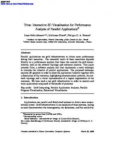
FIGURE 3. Call graph display using tagged objects

around in 3D space. Figure 3 shows a call graph where tagged objects are used to represent the files. In this case there is a small gap between the tag and the layout object, the layout object for the non-selected items is shrunk to the size of the tag and at a 90° angle, and the layout for the selected items is full size and at a 0° angle. • Time Sequences. One of the uses of 3D is to show the history of execution (or any other time-based property of programs) in the Z dimension. Time sequence objects are one way that we have developed for doing this. These consist of a base component which identifies an X-Y position for each object and a set of elements. Each element consists of an object, a from time and a to time, and a reference to an object in the base component. The element is drawn using the X and Y position An Engine for the 3D Visualization of Program Information

May 5, 1995

13

FIGURE 4. Dynamic call graph display using a time sequence object

and size of the referenced base component and using the time properties to set the position and size in the Z dimension. Properties of time sequence objects specify the relative size for a given unit of time and the direction of time. Properties of the component objects are used to specify nesting levels. This is used for recursive function invocations where boxes would be contained in each other. Each increase in nesting level causes the corresponding box to be drawn slightly smaller so that the element boxes nest properly. A time sequence object is drawn by first drawing optional shadows and then drawing the component objects. Shadows, if desired, are drawn as if a light were coming from the top of view, with the shadows appearing in the X-Z plane. Properties allow the setting of the shadow color and transparency. Figure 4 shows a top-down view of a dynamic call graph display using a time sequence object. The layout


May 5, 1995

14

object at the front (bottom) is a 2D representation of the call graph. The yellow boxes behind (above) this object represent dynamic instances of the elements of the call graph. Here time flows backwards (from bottom to top) in Z. • 3D Trees. This 3D representation for a tree is based on cone and cam trees developed at Xerox. Here the children of a node are arranged in a planar circle underneath their parent. While the children are placed at equal intervals around the circle, the radius of the circle and the distance from the parent to the circle are determined based on properties of the parent object. The radius of the circle is determined by finding the minimum radius that will easily contain all the children based on the children’s sizes and then multiplying this by a scale factor specified as a property. The distance from the parent is computed based on properties that specify the angle from the parent to the circle and the minimum allowable height. A property is also used to determine the orientation of the tree. If the up direction is set to Y then the result is a cone tree. If the up direction is set to X, the result is a cam tree. Tree objects are drawn by drawing the components and then connecting the children components to the parent. The connection can be done either as a cone from the bottom of the parent to the top of the children or as lines from the parent to each of the children. The orientation of the circle can be changed by setting a property that causes a selected component to come to the front. An example of a tree layout is shown in figure 5. The third category of presentation styles includes styles that control both layout and presentation. These include: • Scatter Plots. These consist of a rectilinear region with components placed based on three values. Scatter plot components can be arbitrary objects. The scatter plot object computes the range of values in each dimension and finds the associated location for each component. It then places the components accordingly. The properties associated with the scatter plot control the basic size of the region and the size of the components. Figure 6 shows a scatter plot display of a call graph that provides information about the routines. The X dimension reflects the amount of run time spent in the routine (as determined by profiling); the Y dimension represents the length in lines of the routine; and the Z dimension represents the number of other routines that call the routine. • File Objects. The central focus for programming is the source code and many visualizations relate directly to files. Based on SeeSoft ideas developed at Bell Labs, a file object presents an abstract view of a file that can be augmented with additional information to reflect properties associated with regions in the file. A file is represented as a planar region where each line of the file corresponds to one line in the region. If the region is too long, it is divided into columns and the columns placed side by side. The lines are used to represent information about the corresponding portion of the file. Each line can be drawn full width or can be drawn to reflect the indentation and line length of the corresponding text. The latter mode allows identification of program structures, block comments, etc. and allows a programmer who is familiar with the code to associate the representation with the An Engine for the 3D Visualization of Program Information

May 5, 1995

15

FIGURE 5. Tree layout

text. Each line can also be associated with a height and a color value, allowing both color and depth to be used to convey information about that line in the graphical representation. Properties associated with file objects allow the setting of the file name, the width of each line, how the line should be drawn, the width of the border around the lines, the number of lines in a column, and the mapping from data values to depth and color. Figure 7 shows file objects being used in a call graph display. File objects use both components and constraints. Components are used to describe parts of the file that should be treated as units and that can have associated values that are to be reflected in the presentation in terms of color or depth. Each component is identified by a start and end line and an underlying object. While this object isn’t drawn, its properties are used in determining how to draw An Engine for the 3D Visualization of Program Information

May 5, 1995

16

FIGURE 6. Scatter plot display of run time vs. length vs. static entries for a call graph

the corresponding part of the file. Constraints are used to describe the properties that are to be reflected for each component. Each constraint specifies the style property that is affected (i.e. color or depth), the default value, the range of valid values and a scale factor. • Plot Layout Objects. These objects allows the application control over both the layout and sizing of the component objects. It assumes that all the components are to be placed inside a cube of a specified size. Each component can be assigned a size in zero or more dimensions and can be assigned a relative position in any of the axis. If sizes and positions are fully specified for each object, the resultant display is a generalized array. This is useful, for example, in putting up a display of blocks in memory where the Y dimension reflects the page of memory the block occurs in, the X dimension reflects the location within that page, and the Z dimension reflects the lifetime of the block. If sizes are left unspecified, then the component is assigned a standard size based on the number of objects and the size of the overall cube. If positions are left unspecified, then the plot layout object uses a relaxation-based optimization strategy to place nodes. First an initial position is determined. If the object had been drawn before, the previous positions are used here, otherwise nodes are assigned arbitrary positions. Then the layout object makes optimization passes over the An Engine for the 3D Visualization of Program Information

May 5, 1995

17

FIGURE 7. Call graph display showing file objects

objects, adjusting the positions to try to separate unrelated objects and group related ones where relationships are determined by the arcs connecting the objects. The maximum number of optimization passes is set as a parameter, but the optimization stops if the layout stabilizes, which it generally does after about fifty passes. Each pass consists of making objects repel each other using an inverse square force determined by the standard objects size and a parameterized scale factor, and then having related objects attract each other using a force that is proportional to the square of the distance between them where the scale factor is determined by the object size and a object property. A third, optional portion of each pass, allows objects to be attracted or repelled from the walls of the cube based on an object property. This approach is currently O(n2), which means it is not practical for large layouts.


May 5, 1995

18

FIGURE 8. Sample plot layout object of a call graph

Plot objects are drawn by drawing the containing cube, either so that it is hollow of so that the interior is visible, and then drawing the components. Properties allow the arc components to not be drawn, allowing arcs to be used only to specify relationships for layout, and allow node objects to be drawn without text. This allows a plot object to be used to simply express relationships spatially without crowding the diagram with text and arcs. The user can query what each node corresponds to by moving the mouse over that node. Figure 8 shows an example of a plot layout object.


May 5, 1995

19

6. Styles in PLUM Properties serve a variety of functions in specifying the various types of presentation objects. They control the graphical presentation of the objects, specify parameters that control the layout, and provide data to be used in the presentation. As such, it was important that PLUM provide a powerful and convenient mechanism for specifying properties. The basic notion is based on styles. A style is a collection of properties each of which is an attribute-value pair. Properties are grouped into styles as a matter of convenience. It is often the case that a set of different objects will share a common set of properties. Styles allow this set to be specified once and then simply associated with each of the objects. Styles are designed to support standard definitions like this while still allowing properties to be overridden for individual objects. They also are designed so that styles from different sources can be easily merged. This allows a style that is specified for selection to be merged with the default style for an object. Finally, styles are designed to allow the setting of default properties for each flavor of presentation object and for drawing. Styles are implemented as objects where values are determined by object-oriented delegation rather than inheritance. Each style contains a mapping from attributes to values, a pointer to a parent style, and a pointer to an alternate style. The mapping is used to contain the local settings of values for the style. These local settings represent properties that are overridden or defined explicitly in this style. The parent link denotes the style that this style is overriding. If a property cannot be found in the mapping, then the parent style is used recursively to determine the value of an attribute. The alternate style link is used when styles are merged. If a property is not defined in either the local mapping or the parent style, then it is looked up recursively in the alternate style. If two styles are to be merged, a new style is created with the higher priority style specified as the parent link and the other style specified as the alternate link. Styles are used for representing selected presentation objects. Selections are useful when editing (the user selects an object and then an operation on the selected object) and for automatic highlighting (the system could select the currently executing object to provide run time animation). PLUM provides for application-defined selections. Each selection is defined by a selection name and two styles, one for the object that is selected and one for its children. Before a presentation is drawn, a selection style is computed for each presentation object. This is done top down from the root object, with each object providing the default selection style to its children. The default selection style is originally empty. If the object is not selected, it passes the selection style it is given to its children. If the object is selected, then its selection style computed as the merge of style associated with the selection with the inherited selection style. Moreover, the style that it passes to its children is the merge of the style it inherited with the child style of the selection. This scheme allows multiple selections of an object where the different selection styles are merged together.


May 5, 1995

20

Objects have several styles associated with them. In addition to the selection style that is computed by the system, they have a base style that is generally defined by the object to specify default values for object-specific properties, a user style for normal settings, an override style for priority settings, and a child style to indicate settings for their subobjects. The user and override style and properties in these styles can be defined by the application. In order to determine the value associated with an attribute for an object, PLUM considers each of these styles. It first looks the attribute up in the override style. If it is not found there, it looks it up in the selection style that is computed as described above. If it is not found there, it looks it up in the user style. This ordering allows selections to generally override properties of objects while allowing the application to specify object properties that should not be changed by selections. If the attribute is not defined in the user style either, then the child style of the object’s parent object is used. This allows objects to specify default settings of properties for their children that are different from the standard defaults. Next, if the property is not found in any of these styles, the base style for the object followed by the system base style is used. Finally, if the attribute hasn’t yet been found, a system-wide default style is considered. This style is used to specify defaults for the properties that all objects share and that must be specified such as color.

7. Layout Methods in PLUM Most of the work done by the presentation objects involves layout, i.e. placement of subobjects. A variety of different layout strategies are evident, some attempting to use layout to convey information, e.g. using depth to indicate the amount of time spent in a routine or using Z to represent time. Others just attempt to make the layout look “good” according to some abstract criteria. The simplest layout method is used for layout objects and sized layout objects. These methods allow arbitrary nodes and arcs and simply attempt to do graph layout in 3D, typically while presenting a 2D view from the front of the display. Graph layout has been extensively studied in two dimensions [2]. The problem is one of placing nodes and arcs to produce an aesthetically pleasing graph. This is generally translated into more specific problems such as reducing arc length and the number of crossings or of emphasizing symmetry. While we provide a variety of approaches in our 2D layout packages, the algorithm of choice for program data has been one based on level graphs [24] since it tends to emphasize hierarchy and since it generally produces a reasonable looking result. Moving graph layout algorithms from two to three dimensions is not trivial. The first problem is determining what “looks good” in three dimensions. Because 3D graphics imply that the user is going to move around and look at the graph from different perspectives, assumptions based on the user’s view may not be valid. For example, the heuristic of minimizing crossings is meaningless. Given any two arcs in three-space that do not intersect, we can find a perspective where they do not cross and a second perspective where they do cross. Since most arcs will not physically intersect in three space, the number of crossings will vary with the perspective. An Engine for the 3D Visualization of Program Information

May 5, 1995

21

A second problem is that 3-space offers many more degrees of freedom. In two dimensions there are two alternatives to laying out a level graph, representing the levels as either rows or columns, and the resulting graphs are identical except for orientation. In three dimensions one has three alternatives for how to represent levels. Moreover, once the leveling is done, each level can be potentially represented by a plane and hence by an arbitrary 2D layout. One could, for example, apply a 2D level graph algorithm to the remaining nodes, i.e. do leveling twice. Alternatively, the algorithm could place the nodes in a circle as in cone trees. A third problem that arises is that we want to use the third dimension to convey information and not just to provide more space for layout. This means that we have to find layout methods that reflect properties of the underlying objects. For example, layout methods must be able to assign a Z coordinate to a node based on its accumulated run time or what file its in or how distant it is from a set of selected nodes that the user is focusing on. In PLUM we have implemented a flexible approach to 3D layout to experiment with different algorithms and to gain experience with what works and what does not. Our approach allows layout methods to work in various ways. Some methods, such as leveling, work for one dimension and depend on another layout method to handle the remaining dimensions. Other layout methods are comprehensive, working in all three dimensions at once. Still others, such as local optimization, don’t compute the layout in any dimension, but instead modify a layout that is already present. All the layout methods allow values to be defined by the application or by the user. Each coordinate can be given a default relative or a default absolute value. Relative values identify the location in the array that is used by layout objects. These are typically used to represent program assigned values. Absolute values can be used to exactly reflect user manipulations of the underlying objects. All the layout algorithms are also parameterized using properties. The layout methods that handle only one dimension include: • Level graph layout. This layout method handles a single dimension. It computes a leveling of all the nodes that do not have that dimension previously defined and assigns a value in that dimension based on the leveling. Once the leveling is done, a secondary layout method, specified as a property, is applied to handle the remaining dimensions. Properties specify the dimension to be used and whether arcs should be considered directional or not. Other properties control the type of leveling. Normally leveling starts at the root node and assigns each subsequent node a level that is one greater than any of the nodes it is connected to. Bottom-up leveling starts with the leaf nodes. For both of these the level of a node is the maximum of the levels of its predecessors plus one. In breadth-first leveling, the level is assigned on the first visit to the node and not changed. A final property determines whether level heuristics should be applied to the arcs through the insertion of pivot points for the arcs for each level that the arc traverses. This will insure that arcs do not pass through nodes at the cost of having the arcs be crooked.


May 5, 1995

22

• Level ranking layout. This method handles one dimension and assumes that some prior dimension was handled by a level graph layout. It attempts to order the nodes within a level by considering their position relative to the nodes above and below it in the leveling. This is done by making multiple passes over the leveling, alternating top-down with bottom-up, and assigning the positions within each level to minimize arc length. The properties of level ranking layout specify the dimension to work on, the dimension of the previous leveling, the layout method to apply next for further dimensions, and the number of passes that should be made over the graph. • Unique value layout. This method handles one dimension, assigning a unique value to each node in that dimension using a modified depth-first search algorithm. This is useful, for example, to assign a unique Z position for each file grouping in a call graph layout. The properties here set the dimension to be used, the subsequent layout method, and the first value to be used in the dimension. • Value layout. This method handles one dimension based on data associated with each node. It finds the maximum and minimum data values and then places each node in a position relative to its value. Properties allow the position to be determined directly from the data or from the log of the data and allow the data to be interpreted in increasing or decreasing order. Figure 9a shows a random graph of 20 nodes drawn using level graphs in X, level ranking in Y, and unique value in Z. Figure 9b shows the same graph using the node number for a value layout in Z. Other layout methods handle all remaining dimensions. These can be used as a toplevel method or as a secondary method to some of the above to fill in the remaining values. They include: • Depth first layout. This comprehensive (all dimensions) approach is quite simple. It does a depth first search through the graph, visiting each node once. As each node is visited it is placed as close to its parent as possible. Properties here determine whether arcs are considered directional for the depth first search, whether the graph should be laid out in two or three dimensions, and what layout directions are preferred, i.e. down and then to the right. • Breadth first layout. This is similar to depth first layout except that a breadth first search is used in place of a depth first search. • Averaged layout. This is a slightly more sophisticated version of the above. The nodes are looked at in order, either the order they were defined in or a depth or breadth first search order. When a node is considered, the locations of all nodes connected to it that have been previously placed are averaged together to get a target location. Then the new node is placed as close as possible to this target location. The properties of this layout strategy determine the search order, specify whether the layout should be two or three dimensional, and determine the preferred direction for the layout. An example can be seen in Figure 9c.


May 5, 1995

23

a) Leveling with unique Z

b) Leveling with value-based Z

c) 3D averaged layout

d) Optimized 3D average layout

FIGURE 9. Different layout methods illustrated on a random graph

• Orthogonal layout. This layout method attempts to display multiple hierarchies simultaneously using the three dimensions. The primary hierarchy is displayed in the XY plane. Secondary hierarchies can be displayed in the XZ or the YZ plane. The individual hierarchies are laid out using a level graph approach. The method works in one dimension at a time. First the primary hierarchy is used to determine levels in the Y direction. Levels can be determined using either top-down or An Engine for the 3D Visualization of Program Information

May 5, 1995

24

bottom-up leveling. Next the YZ hierarchy, if defined, is used to determine the Z coordinate by leveling and then the XZ hierarchy is used to determine the X coordinate. A node’s position in a hierarchy is determined by associating a hierarchy type with each arc. Finally, any values that have not been defined by the above leveling passes are set using a modified level ranking approach. Finally, we currently provide one post-processing optimization: • Local optimization. This is a post-processing approach that takes a complete layout and applies an optimization algorithm to it. The optimization approach is to assume a linear attractive force between connected nodes and an inverse square repulsive force between nodes that are not connected. Then a relaxation algorithm is employed to find the resultant positions of the nodes. Properties here specify the method that provides the initial layout, the value of the attractive and repulsive forces, and the number of passes to be made in the relaxation algorithm. Figure 9d shows the optimized layout of Figure 9c.

8. Animation in PLUM One of the key features provided by PLUM is automatic animation. Animation is necessary for 3D visualization on a 2D screen. PLUM provides animation in two ways. The simpler is to allow the user to move the camera position so as to fly through the object. The more complex allows arbitrary changes to the presentation objects to be made. The result of the draw phase in PLUM is a display list. This is a hierarchical set of graphical commands such as transform, set property (i.e. color), and draw shape. This list is then traversed to actually render the graphics. Changing the camera position is done by changing one element in the display list and then retraversing it. Where possible, this is done using double buffering to provide a smooth transition from one frame to another. PLUM is designed to be used by an application in an edit-display cycle. The application first sets up a top level presentation object and then asks that it be displayed. Then, in response to a user request or a program action, it either edits the current presentation objects or creates a new top level presentation object. Editing can involve setting new property values for the presentation objects, creating new presentation objects and attaching them as components of existing objects, removing object components, adding or modifying constraints, or selecting or deselecting objects. Once a series of edits is complete or a new top level object has been defined, the application informs PLUM that the edit is complete. Unless told otherwise, PLUM will attempt to animate the transition from the current display to the display of the modified objects. The first stage in this automatic animation process involves identifying what has changed. Each presentation object maintains a flag indicating its current state. This state can be RAW, SIZE_DONE, LAYOUT_DONE, DRAW_COMPUTED, and An Engine for the 3D Visualization of Program Information

May 5, 1995

25

DRAW_DONE. This state indicates what information associated with the object can be preserved. When a property is changed on an object, the state of the object is reset accordingly. The second phase occurs at the start of updating the display. Here PLUM attempts to match old and new objects and to save the old display settings for matched objects. Objects are matched using a compare routine that can be specialized to the different flavors of objects. The basic routine checks if the two objects have the same flavor and the same associated user data value. If two objects match in this sense, the compare algorithm attempts to match components of the two. Components are matched with a preference for order but will handle arbitrary insertions or deletions into the list of components of the original object. This pass also can change the state of each object according to whether it matches a previously known object (where the values are copied) and according to the state of its children. Because the screen is to be redrawn, no object is left in state DRAW_DONE or DRAW_COMPUTED. Once the old and new objects have been compared, PLUM computes the new presentation. When computing size, it will skip any objects whose state indicates that the size has already been computed. Similarly, when computing layout it will skip objects where the layout is already done. The new presentation is then drawn by making passes over the resultant object structure to compute the display list corresponding to each object. Each pass corresponds to one animation frame. The pass is parameterized by a fraction which ranging from 0 (old object) to 1 (new object). The drawing routines for each flavor construct a draw object using properties that are gathered from the object. PLUM provides facilities to inquire the size, the transformation, and properties such that the value returned is a linear combination of the original and new value based on the frame parameter. The property inquiry routines handle standard properties that are known to be numeric (such as transparency) using linear interpolation. They handle standard color properties by interpolating a color in RGB coordinates. All other properties are assigned the new value. The drawing routines (and the extra DRAW state) are set up so that each frame other than the first can change the drawing by simply editing the display list rather than recreating it entirely.

9. Experience with PLUM We have been working on PLUM and the related packages for abstraction visualization for about two years. During that time we have rewritten most of PLUM at least once in attempting to find the proper abstractions and interface. The current system comprises about 25,000 lines of C++ code and is built on top of a machine-independent graphics library provided by the Brown University graphics group. Much of our experience with PLUM has been positive. The framework provided by PLUM makes it easy to add new presentation styles. This is due to the use of hierarchy to simplify what each presentation has to do, the general notions of properties, An Engine for the 3D Visualization of Program Information

May 5, 1995

26

components and constraints that are supported by the system. We have been able to integrate a variety of different presentations into this framework in a natural way. Adding a new presentation style can generally be done in a day or less, but additional time is often required to fine tune the graphical presentation. The interface between PLUM and the application also seems to be the right one. The application defines objects, components, and constraints. Styles and properties are associated with objects. Properties can be set for components and constraints. Because object, components, constraints, and styles are all generic, the size of the interface that is required is quite small given the complexity of the system. The use of automatic animation allows the application to compute the new presentation without having to specify how it differs from the old. This often greatly simplifies the application. In addition to using PLUM as a back end for visualizing program information gathered by the FIELD environment (i.e. call graphs, the class hierarchy, and profiling information), we have also used it to display the results of program performance analysis in a separate system. This tool, vprof, provides three different 3D displays: a file view showing how much time is spent at each line and how often that line is executed, a scatter plot of functions showing total instruction vs. local instructions vs. real time, and an abstraction of the dynamic call graph showing where the program spends its time. An example of the latter is shown in Figure 10. Here the size of the block in XZ is proportional to the allocated run time; the position indicates its place in the call hierarchy; the color indicates its ranking it terms of total run time; its Z height up indicates the amount of real time spent in the routine; and the Z height down indicates the number of times the routine was called. The total code needed in vprof to provide the three interfaces was around 1000 lines. The major drawback to the current implementation of PLUM is its performance. This is partially due to the inefficient way we currently use the native graphics hardware on the Suns, to the fact that we are using interprocess communications for communicating data from the application to PLUM, and to the size of the storage structures created in the browser. Our current implementation is practically limited to working with under 50,000 objects and displaying only a hundred simultaneously. We are attempting to design the next generation system to handle a million objects.

10. Conclusions Practical program visualization requires a flexible back end that is capable of providing a wide variety of different visualizations. Different aspects of the program need to be visualized in different ways. Moreover, different presentation methods will be needed by the user to understand and gain insight into different program understanding tasks. The back end must provide advanced capabilities both to help the user in viewing large amounts of data and to simplify the application interface. These capabilities include a convenient user interface for flying around and viewing the result, automatic layout and routing where appropriate, constraint-based layout An Engine for the 3D Visualization of Program Information

May 5, 1995

27

FIGURE 10. Performance display showing abstract dynamic call graph

and presentation styles, and automatic animation from one frame to the next so that the user does not lose context as the display changes. PLUM is our attempt to provide such a back end. We feel that PLUM successfully meets these criteria. It provides a very simple program interface based on objects, components, constraints and properties that can be used by an application with a minimum of effort. This is demonstrated both in our initial implementation to display FIELD program data, in a 1000 line program that displayed a 3D representation of semantic nets, and in the 1000 lines added to our performance tool to provide three different graphical displays. We expect to use the system in several other visualizations and to release it to other researchers in the future.


May 5, 1995

28

11. References 1. David B. Baskerville, “Graphic presentation of data structures in the DBX debugger,” UC Berkeley UCB/CSD 86/260 (1985). 2. G. Di Battista, P. Eades, R. Tamassia, and I. G. Tollis, “Algorithms for drawing graphs: an annotated bibliography,” Comput. Geom. Theory Appl Vol. 4 pp. 235-282 (1994). 3. Marc H. Brown and Robert Sedgewick, “Techniques for algorithm animation,” IEEE Software Vol. 2(1) pp. 28-39 (1985). 4. Marc H. Brown and John Hershberger, “Color and sound in algorithm animation,” Computer Vol. 25(12) pp. 52-63 (December 1992). 5. Marc H. Brown and Marc A. Nojork, “Algorithm animation using 3D interactive graphics,” DEC Systems Research Center (1992). 6. Jacques Davy, “GoPATH programmer’s guide,” Bull Imaging and Office Solutions (December 1992). 7. Stephen G. Eick, Joseph L. Steffen, and Eric E. Sumner, Jr., “Seesoft - a tool for visualizing software,” AT&T Bell Laboratories (1991). 8. Belinda B. Flynn and David Maier, “Specification and generation of displays for complex database objects,” Oregon Graduate Institute of Science and Technology (1992). 9. Sadahiro Isoda, Takao Shimonmura, and Yuji Ono, “VIPS: a visual debugger,” IEEE Software Vol. 4(3) pp. 8-19 (May 1987). 10. Clinton Lewis Jeffrey, “A framework for monitoring program execution,” U. Arizona Technical Report TR 93-21 (July 1993). 11. Hideki Koike, “The role of another spatial dimension in software visualization,” ACM Trans. on Info. Sys. Vol. 11(3) pp. 266-286 (July 1993). 12. Mark A. Linton and John M. Vlissides, “Unidraw: a framework for building domain-specific graphical editors,” Proc. UIST ’89, pp. 158-167 (November 1989). 13. Jock D. Mackinlay, George G. Robertson, and Stuart K. Card, “The perspective wall: detail and context smoothly integrated,” Proc. CHI’91, pp. 173-179 (April 1991). 14. Brad A. Myers, “Incense: a system for displaying data structures,” Computer Graphics Vol. 17(3) pp. 115-125 (July 1983). 15. Brad A. Myers, Dario A. Guise, Roger B. Dannenberg, Brad Vander Zanden, David S. Kosbie, Edward Pervin, Andrew Mickish, and Philippe Marchal, “Garnet: comprehensive support for graphical, highly interactive user interfaces,” IEEE Computer, pp. 71-85 (November 1990). 16. Michael L. Powell and Mark A. Linton, “Visual abstraction in an interactive programming environment,” SIGPLAN Notices Vol. 18(6) pp. 14-21 (June 1983).


May 5, 1995

29

17. B. A. Price, I. S. Small, and R. M. Baecker, “A taxonomy of software visualization,” Journal of Visual Languages, (Dec. 1993). 18. Steven P. Reiss and Joseph N. Pato, “Displaying program and data structures,” Proc. 20th Hawaii Intl. Conf. System Sciences, (January 1987). 19. Steven P. Reiss, “Working in the Garden environment for conceptual programming,” IEEE Software Vol. 4(6) pp. 16-27 (November 1987). 20. Steven P. Reiss, Scott Meyers, and Carolyn Duby, “Using GELO to visualize software systems,” Proc. UIST ’89, pp. 149-157 (November 1989). 21. Steven P. Reiss, “Connecting tools using message passing in the FIELD environment,” IEEE Software Vol. 7(4) pp. 57-67 (July 1990). 22. Steven P. Reiss and Manojit Sarkar, “Generating program abstractions using an object-oriented database,” Brown University Department of Computer Science (1992). 23. George G. Robertson, Jock D. Mackinlay, and Stuart K. Card, “Cone trees: animated 3D visualizations of hierarchical information,” Proc. CHI’91, pp. 189-194 (April 1991). 24. L. A. Rowe, M. Davis, E. Messinger, C. Meyer, C. Spirakis, and A. Tuan, “A browser for directed graphs,” Software Practice and Experience Vol. 17(1) pp. 61-76 (1987). 25. Manojit Sarkar, Scott S. Snibbe, Oren J. Tversky, and Steven P. Reiss, “Stretching the rubber sheet: a metaphor for viewing large layouts on small screens,” Proc. ACM SIGGRAPH UIST, pp. 81-91 (November 1993). 26. Manojit Sarkar and Marc H. Brown, “Graphical Fisheye Views,” CACM Vol. 37(12) pp. 73-84 (December 1994). 27. John T. Stasko, “TANGO: a framework and system for algorithm animation,” IEEE Computer Vol. 23(9) pp. 27-39 (September 1990). 28. James Wen, “A three dimensional browser for visualizing orthogonal hierarchies,” Brown University (1992).


May 5, 1995

30