Iranian Journal of Science & Technology, Transaction B, Engineering, Vol. 31, No. B1, pp 13-30 Printed in The Islamic Republic of Iran, 2007 © Shiraz University
AN ENGINEERING INVISCID-BOUNDARY LAYER METHOD FOR CALCULATION * OF AERODYNAMIC HEATING IN THE LEEWARD REGION M. MAEREFAT1,** S.M.H. KARIMIAN2 AND M. MALEKZADEH DIRIN1 1
Dept. of Mechanical Engineering, Tarbiat Modares University, Tehran 14115-111, I. R. of Iran Email:
[email protected] 2 Dept. of Mechanical Engineering, Amirkabir University of Technology, Tehran 15914, I. R. of Iran Abstract– An engineering method has been developed for the prediction of aerodynamic heating of hypersonic bodies. This method is capable of rapidly predicting the heat flux in the leeward region. This is achieved through the determination of the streamlines in the leeward region. The modified form of Maslen’s second order relation is employed, which calculates the pressure in the shock layer explicitly. The inviscid outer flow within the shock layer is solved first. The calculated solution is then used to determine the flow properties at the boundary layer edge and the orientation of the surface streamlines. Boundary layer equations, written in the streamline coordinates, are integrated along the surface to obtain the rate of heat transferred to the body surface. The present method is an inverse method in which the body shape is obtained according to the shape of the shock. In general, inviscid-boundary layer engineering methods accurately calculate the orientation of streamlines in the windward region only, and therefore they are not usually applicable in the leeward region. In the present study, a new method is proposed to determine the orientation of the surface streamlines in the leeward region. Using the present technique, three-dimensional hypersonic flow is solved fast and easy all around a cone. The obtained results show that the corrections presented in this study excellently extend the application of the method to the leeward region. Keywords– Inviscid boundary layer, hypersonic flow, aerodynamic heating, numerical simulation
1. INTRODUCTION An accurate prediction of convective heat transfer is necessary for efficient thermal design of a hypersonic vehicle. To achieve this, various numerical methods can be used to solve the flowfield around the vehicle. These methods are mainly based on CFD techniques which solve Navier-Stokes (NS) equations [1] or one of their simplified versions [2, 3]. However, they are not applicable for rapid estimation and design [4], as they are rather time consuming and require special computing facilities. Methods based on approximate thin layer assumptions are widely used for calculations of aerodynamic heating in hypersonic flow fields [5]. In these methods, the flowfield is divided into two regions: the boundary layer region, and the inviscid outer region. First, the inviscid flow is solved and the flow properties obtained on the body surface are then taken as properties at the edge of the boundary layer. The viscous flow inside the boundary layer can now be solved to determine the convective heat flux at the body surface. To determine the properties of the inviscid flowfield within the shock layer, the Maslen method can be used. Although Maslen's original method [6] was developed for axisymmetric hypersonic flow, Maslen improved his method to cover threedimensional flows as well [7]. The outcome of the Maslen method is a second order relation from which pressure can be calculated explicitly in a direction normal to the shock. Using other conservation equations, the flowfield within the shock layer is calculated. Depending on the shock shape, the body ∗
Received by the editors May 13, 2003; final revised form October 30, 2006. Corresponding author
∗∗
14
M. Maerefat / et al.
geometry is determined from the solution, therefore the method is an inverse one and an iteration procedure would be necessary. However, difficulties have been encountered in many cases where this method has been used [5]. Recently, Riley and DeJarnette [8-10] developed a three-dimensional approximate method which is applicable to a wider range than that applied by Maslen's axisymmetric method. Their method is similar to that proposed by Jackson [11] for smooth symmetric bodies. They have used a modified form of Maslen’s second order relation for pressure. Since this method predicts the pressure on the body surface with good accuracy, the surface streamlines are calculated using pressure distribution. Obviously, Riley and DeJarnette's method is also an inverse one. Using axisymmetric analog [12], three-dimensional boundary layer equations along the streamlines are reduced to an axisymmetric form. The obtained equations are integrated along the streamlines to determine the rate of heat flux on the body surface [13]. However, the latter method is not yet capable of predicting streamlines along the body in the leeward region. Therefore, the boundary layer equations cannot be solved in this region. The goal of the present work is to modify this method in order to be applicable to the leeward region of blunt-nosed bodies. For this purpose, a linear approximation between the streamlines of φ b = 90 degree and φ b = 180 degree is employed to estimate the orientation of surface streamlines in the leeward region. In the following sections the principles of the method and the proposed corrections are presented. 2. INVISCID ANALYSIS The present method is an inverse one, meaning given an initial shock shape, flow equations in the shock coordinate system are solved to determine the corresponding body geometry. Therefore, we introduce the shock coordinate system first. a) Coordinate system Before introducing the shock coordinate system, it is mentioned that the surface of a threedimensional shock [14] can be described in a cylindrical coordinate by
r = f ( x ,φ
)
(1)
( x , r ,φ ) are wind-oriented cylindrical coordinates, and the corresponding unit vectors are ( e x , e r , e φ ) . The x-axis is aligned with the freestream velocity vector, and it is normal to the shock surface in the origin of the coordinate system. The shock shape is described by two angles; Γ( x, φ ) and δ φ ( x, φ ) , which are defined as follows: ∂f 1∂f tan δ φ = tan Γ = cos δ φ (2) f ∂φ ∂x where
The other angle σ is simply defined as σ = φ − δ φ . The angles and coordinate system are shown in Figs. 1 and 2. The shock-oriented curvilinear coordinate system ( ξ , β , n ) is defined [14], with ξ and β as coordinates of a point on the shock surface, and n as the inward distance normal to the shock. The unit vector en is in the inward direction normal to the shock. The unit vectors eξ and e β are tangent to the surface of the shock, so that eξ is in the direction of velocity tangent to shock, and e β is normal to the vectors eξ and en (Figs. 3 and 4). The unit vectors in a curvilinear shock-oriented system [15] are related to the unit vectors in cylindrical coordinates as follows:
eξ = cos Γ e x + sin Γ cosδ φ er − sin Γ sin δ φ eφ e β = sin δ φ er + cos δ φ eφ
(3)
Iranian Journal of Science & Technology, Volume 31, Number B1
February 2007
An engineering inviscid-boundary layer method for…
15
en = sin Γ e x − cos Γ cos δ φ er + cos Γ sin δ φ eφ For the sake of clarity, β constant lines are shown in Figs. 3 and 4. The velocity vector in the shock layer is given by
r V = u eξ + v en + w eβ
(4)
Considering definitions of e β and eξ , the cross flow velocity at the shock ( ws ) is found to be equal to zero.
Fig. 1. Shock wave geometry: rear view
Fig. 2. Shock wave geometry: side view
Fig. 3. Shock oriented curvilinear coordinate system: side view
Fig. 4. Shock oriented curvilinear coordinate system: rear view
b) Governing equations For a blunt-nosed body in hypersonic flows, most of the mass flow passes through the vicinity of the shock where velocity component w is negligible [6, 7]. Therefore, the governing equations for inviscid three-dimensional flow in a shock layer can be simplified by taking w = 0 . With this assumption and using the continuity equation, the stream function is defined as
∂ψ = ρ v hξ hβ AB ∂ξ
∂ψ = − ρ u hβ B ∂n
(5)
where ρ is density, hξ and hβ are scale factors, and A and B are geometric factors. Now, the continuity ~ ~ and normal momentum equations are transformed to the stream function coordinate system ( ξ , β ,η ), in which February 2007
Iranian Journal of Science & Technology, Volume 31, Number B1
M. Maerefat / et al.
16
~
~
ξ =ξ
β =β
η =ψ ψ s
To obtain approximate expressions for the pressure and the normal velocity component, the following thin shock layer assumptions [6, 7] are used
ρ ≈ ρs
A≈1 B≈1 ∂ vs ~ ≈0 ∂ξ
u ≈ us ∂ ρs ~ ≈0 ∂ξ ⎛ ∂n ⎞ n ≈ ⎜⎜ ⎟⎟ (η − 1) ⎝ ∂η ⎠ s
Integrating the obtained equations gives the following expressions [9]:
(
)
(
)
(
)
~ ~ ~ ~ p ξ , β ,η = ps ξ , β + p1 (η − 1) + p2 η 2 − 1
(
) (
(6)
)
~ ~ ~ ~ v ξ , β ,η = vs ξ , β + v1 (η − 1) where
p1 = p2 = v1 =
ψ s u s kξ hβ
ψ s v s tan Γ 2 hβ
ψ s vs hβ cos Γ
(kξ + k β )
(7)
( kξ + k β )
and k ξ and k β are the curvatures of the shock surface in ξ − η and β − η planes, respectively. For a prescribed shock shape, the quantities p1 , p2 and v1 in Eqs. (6) and (7) are known, and therefore they can be used to explicitly determine the pressure and the normal component of velocity in the shock layer. Having known the pressure, other quantities such as density and enthalpy can be found using isentropic relations and ideal gas equations of state. The tangent velocity component, u, is found from the conservation of total enthalpy. Another important relation which is obtained by integrating Eq. (5) is 2
nb −
nb k β
2
=
ψs hβ
∫
dη 0 ρu 1
(8)
From this relation the normal distance between the shock and the body can be obtained. c) The inviscid flow solution
The inviscid solution is obtained for a given shock shape. Therefore, the shock shape should be changed so that the calculated inviscid solution corresponds to the body shape. This iterative process is performed differently in the two regions of subsonic and supersonic. In the stagnation region around the blunt nose of hypersonic bodies, the flow is subsonic, and due to the elliptical behavior of the flow, the shock shape should be known completely in this region. In this region, a three-dimensional shock shape is estimated from the three longitudinal conic sections blended in the circumferential direction with an ellipse [9]. The longitudinal conic sections are given by [16]. Iranian Journal of Science & Technology, Volume 31, Number B1
February 2007
An engineering inviscid-boundary layer method for…
f k + bk x 2 − 2 c k x + 2 d k x f k = 0
17
k = 1,2,3
2
where f k is the radial coordinate of the equation, and k denotes the situations corresponding to β = 0 ,90 ,180 . The elliptic surface generated from these three equations is
[
]
~ ~ ~ f 2 B ( x) cos 2 φ + sin 2 φ + f C ( x) cos φ = D( x)
(9)
where
f2 ~ B ( x) = 2 f1 f 3 ~ ~ C ( x) = B ( x)( f 3 − f1 ) ~ D( x) = f 22 Equation (9) includes nine constants (bk , c k , d k ) . The shock curvature at the origin is continuous in the planes of symmetry. Therefore, c1 = c3 . Applying the symmetry condition with respect to the x-y plane for the shock shape (Fig. 1), we will find that d 2 = 0 and d1 = − d 3 . Thus the nine unknown constants are reduced to six unknowns. Therefore, it is these six constants that should be changed so that the body shape obtained from the inviscid solution conforms to the actual body shape at six locations. Details of the method are given in [16]. At the end of the subsonic region the flow becomes entirely supersonic, and a marching technique may be used. The relations concerning the shock variables are given [9] as follows:
∂r = sinΓ cosδφ ∂s
∂x = cos Γ ∂s sin Γ cos δ φ ∂φ =− ∂s r ∂ψ s = hβ sin Γ ∂s
∂ sin Γ = − kξ cos Γ ∂s ∂ hβ ∂s
(10)
= hβ k β tan Γ
By integrating the above equations along the shock lines, shock variables including ( x, φ , r , sin Γ, hβ , φ s ) will be found. For this purpose, solutions at the end of subsonic flow are used to start the supersonic solution. The shock variables are extrapolated in ξ along β lines. By using Eqs. (6) and (7), on each line, the pressure and the normal velocity component are found. The quantities of enthalpy and density of the flow are also found from isentropic relations, together with the ideal gas equation of state. The tangent velocity component, u, is obtained from the fact that the total enthalpy is constant
1 H = h + ( u 2 + v2 ) 2
(11)
At the present stage, all flow properties are already determined in the region from the shock ( η = 1 ) to the body ( η = 0 ). Therefore, the distance between the shock and body could be found from Eq. (8). If the calculated body does not correspond to the actual body shape, the shock curvature kξ is corrected by the second method, and the solution procedure is repeated. Usually two or three iterations are sufficient. In the subsonic region the same geometric relations are used, however since the shock shape is already known, there is no need to estimate kξ . In the subsonic region geometric relations are integrated along the shock lines of β = 0,90,180 . The shock geometric relations, Eq. (10), became singular at the stagnation point, therefore a limiting form of these relations should be used in this region. Details of the solution for the stagnation point are given in [16]. February 2007
Iranian Journal of Science & Technology, Volume 31, Number B1
M. Maerefat / et al.
18
3. VISCOUS FLOW SOLUTION
Boundary layer equations should be solved for the calculation of aerodynamic heating, however to save computation time, axisymmetric analog is used. a) Axisymmetric analog
With axisymmetric analog, three-dimensional boundary layer equations are simplified so that they can be used in the streamlines direction [12]. In this analysis the three-dimensional boundary layer equations are written in the streamline coordinate system defined on the surface, and then the velocity component tangent to the surface and normal to the streamlines is set equal to zero. This simplifies the threedimensional boundary layer equations to their axisymmetric form in the streamline direction, provided that the distance along the streamline is substituted for the surface distance and the scale factor describing the divergence of the streamlines is interpreted as the axsiymmetric body radius. Thus ds = hξ dξ , r = hβ b) Inviscid streamlines
The inviscid flow streamlines on the body surface should be determined before applying the axisymmetric analog. For this purpose the pressure distribution on the body surface [15] or the velocity components on the surface [17] may be used. Since the present method is more accurate in predicting surface pressure, streamlines will be calculated from surface pressure distribution. To perform this, the coordinate system ( ξ , β , n ) along the streamlines is introduced [15]. Coordinates ξ , and β are coordinates of a point on the body surface, and n is normal distance from the surface. In this coordinate system, eξ is along the streamlines and tangent to the body surface, eβ is normal to the streamlines and tangent to the body, and en is normal to both eξ and eβ . The bars indicate that the coordinates are related to the body, not to the shock. If the body surface is defined as rb = f ( x ,φ ) in the cylindrical coordinate, the unit vector normal to the surface (outward) will be given by
en = − sin Γ e x + cos Γ cos δ φ er − cos Γ sin δ φ eφ where the body angles are defined as
tan δ φ =
1∂f f ∂φ
tan Γ =
∂f cos δ φ ∂x
The vectors tangent to the surface i.e. eξ and eβ , which are similar to eξ and eβ , are defined [15] by
eξ = cosθ e s + sin θ et
(12)
e β = − sin θ es + cosθ et
(13)
where
es = cos Γ e x + sin Γ cos δ φ er − sin Γ sin δ φ eφ et = sin δ φ er + cos δ φ eφ and θ denotes the angle between streamlines and e s . Therefore, if θ is determined all around the body surface, the streamlines would be determined on the surface, because the s and t directions depend on the body direction and eξ is in the streamline direction (Fig. 5). The streamlines direction on the body surface, or θ , are determined by applying momentum equations along the body surface using pressure Iranian Journal of Science & Technology, Volume 31, Number B1
February 2007
An engineering inviscid-boundary layer method for…
19
distribution obtained from the inviscid solution [10]. Writing the momentum equations in the streamline coordinates, taking their scalar product with eβ , and substituting the unit vectors from Eqs.(12) and (13), results in the equation
1 ∂θ sin Γ ∂ σ 1 1 ∂ pb =− − 2 hξ ∂ ξ hξ ∂ ξ ρ b u b hβ ∂ β
(14)
where σ = φ − δ φ . The other equation that should be solved together with the above equation to find scale factor hβ , is obtained using the following relation, which is valid for an orthogonal coordinate system
∂ ∂ ( hβ e β ) = (h e ) ∂ξ ∂β ξ ξ
Fig. 5. Schematic streamline direction
Taking the scalar product of this equation with eβ and replacing the unit vectors in it [10], would result in
1 ∂ ( ln hβ ) 1 ∂ θ sin Γ ∂ σ = + hξ ∂ξ hβ ∂ β hβ ∂ β
(15)
Therefore, to determine the quantities of θ and hβ , Eqs. (14) and (15) should be integrated along the streamlines. This can be done after solving the inviscid flow, however this makes the solution process slow and complicated. Therefore, it is preferred to transform these equations from the streamline coordinates to the shock coordinates system [10]. The transformation relations are
J ∂ 1 ∂ 1 ∂ + (− D eξ . eξ + A eξ . e β ) = ( B eξ . eξ − D eξ . e β ) hξ ∂ ξ hξ ∂ ξ hβ ∂ β
(16)
J ∂ 1 ∂ 1 ∂ + (− D e β . eξ + A e β . e β ) = ( B e β . eξ − D e β . e β ) hβ ∂ β hξ ∂ ξ hβ ∂ β
(17)
where
A = 1 − nb k ξ
B = 1 − nb k β
nb ∂ Γ hβ ∂ β
J = A B − D2
D=
Unfortunately, the pressure relation (Eq.(6)) is not accurate in the leeward region, since this relation is obtained using thin shock layer assumption and the shock thickness is not thin in this region. Thus, it is February 2007
Iranian Journal of Science & Technology, Volume 31, Number B1
M. Maerefat / et al.
20
not possible to calculate the orientation of the surface streamlines from the surface pressure distribution. In other words, Riley and DeJarnette's method is not applicable in the leeward region [10]. Furthermore, in the above-mentioned operators the derivatives with respect to n have been neglected. This is acceptable when the normal to the shock unit vector en is in the same direction of the normal to the body unit vector en , i.e. en = −en . Otherwise the following two terms should be added to the operators of 16 and 17 respectively.
(eξ . en )
∂ ∂n
and
(e β . e n )
∂ ∂n
In some cases the shock is approximately parallel to the body, and we can assume en ≅ −en . In this case
(eξ . en ) = − (eξ . en ) = 0 (e β . e n ) = − (e β . e n ) = 0 In other cases the above relations are not correct. For example, when the body has an angle of attack, although the unit vectors normal to the body and normal to the shock are parallel in the windward region, they are not parallel in the leeward region (Figs. 6 and 7). Therefore, these incomplete operators may affect the accuracy of the streamline directions in the leeward region.
Fig. 6. Shock wave and body geometry: side view
Fig. 7. Shock wave and body geometry: rear view
In the present study, a linear interpolation for determining the streamline direction in the leeward region is proposed. The proposed approximation is obtained by studying the actual physical situation of the flow. All streamlines passing from windward to the leeward are approximately parallel at φ b = 180 degrees. Since the direction of streamline which passes through (or near) φ b = 180 degrees is known ( θ φb =180 = 0 ), in the leeward region, a linear interpolation between θ φb =90 and θ φb =180 may be used in order to estimate the streamline direction. i.e.
⎛ −1 ⎞ φb + 1 ⎟ π ⎠ 2⎝
θ = 2θ π ⎜
π 2
p φb p π
This approximation is compatible with the actual physical situation. Note that, the streamlines direction in π the windward region ( 0 p φb p ) is determined from Eqs. (14) and (15). In the results section it will be 2 verified that the present correction enables the method to be applied to the leeward region. c) Convective heat transfer equations
The heat transfer rate on the surface is found using the Stanton (St) number defined as Iranian Journal of Science & Technology, Volume 31, Number B1
February 2007
An engineering inviscid-boundary layer method for…
St =
21
qw ρ e u e (haw − hw )
where haw is the adiabatic wall enthalpy. Using Reynolds analogy, a correlation between Stanton number St, skin friction coefficient C f , and Prandtl number Pr is obtained as
Cf
St =
2
(Prw ) − m
For laminar or turbulent flow, C f could be calculated from the following relation [16]:
Cf 2
= c1 (Reθ ) − m
where Reθ is the Reynolds number based on the momentum thickness, and c1 and m are constants for laminar flow. This relation is applicable to incompressible flows, and for compressible flows, the reference enthalpy method explained in [18] may be used. According to this method, if all physical quantities of the flow are determined at a reference enthalpy or temperature, then relations of the incompressible flow can be used for compressible flow calculations. The reference enthalpy is defined as
h∗ =
1 (he + hw ) + 0.22(haw − he ) 2
Zoby [13] used the axisymmetric analog together with the Reynolds analogy and reference enthalpy method, to develop the following relations for the calculation of the heat transfer rate. These relations are obtained from an approximate integral solution of boundary layer equations in the streamline direction. For laminar flow
ρ∗ µ∗ )( ) ρ e u e (haw − hw )(Prw ) −0.6 ρe µe
qWL = 0.22(ReθL ) −1 (
(18)
1
0.664( ∫ ρ ∗ µ ∗ ue hβ dξ ) 2 ξ
θL =
0
(19)
ρ e ue hβ
For turbulent flow
qWT = c1 (ReθT ) −m (
ρ∗ µ∗ m )( ) ρ e u e (haw − hw )(Prw ) −0.4` ρe µe ξ
θT =
(c 2 ∫ ρ ∗ µ ∗ u e hβ 3 dξ ) c4 m
(20)
c
0
(21)
ρ e u e hβ
where the constant coefficients are defined [13] by
m=
2 N +1
c3 = 1 + m
⎡ ⎤ N 1 c1 = ( ) N +1 ⎢ ⎥ c5 ⎣ ( N + 1)( N + 2) ⎦ 2N
February 2007
m
c4 =
1 c3
Iranian Journal of Science & Technology, Volume 31, Number B1
M. Maerefat / et al.
22
c 2 = (1 + m) c1
N = 12.67 − 6.5 log(ReθT ) + 1.21[log(ReθT )]
c5 = 2.2433 + 0.93N
2
d) Viscous solution method
Equations 14 and 15 are transformed to the shock coordinate system, and then together with the geometric relations (Eq. (10)) are integrated along the shock lines in the windward region to determine the θ and hβ quantities. In the leeward region θ is obtained from a linear relation which was previously explained, however, hβ is obtained from the solution of Eq. (15). Note that Eqs. (14) and (15) are solved after correcting the shock shape in the subsonic region. Having determined hβ , the integral Eqs. (19) and (21) are solved to obtain the momentum thickness θ . These equations are also transformed to the shock coordinate system before being solved. The momentum thickness is used to determine the Reynolds number based on this thickness, i.e. Reθ . Now Eqs. (18) and (20) are employed to calculate heat transfer rate. Further details are given in [16]. 4. RESULTS
In this section, surface heating rates are calculated over a blunt cone at angle of attack in perfect gas laminar flow. The application of our method is not confined to the ideal gas assumption, and any equation of state of the gas may be used. Note that the results are shown in nondimensional quantities. Solutions are described in a body-oriented coordinate system ( x , r ,φ ) at the circumferential locations of φ b = 0 degree and 180 degrees which are along the windward and leeward sides of the plane of symmetry respectively. The distance along the surface is nondimensionalized by nose radius. In the first case, air flow around a cone of 15 degree half angle and spherical nose radius of 0.0279 m is solved. Surface temperature is Tw = 300° K, angle of attack is 10 degrees, and freestream properties are M ∞ = 10.6, T∞ = 47.3° K , ρ ∞ = 0.00973 kg m 3 . In Figure 8 the results for heat flux in the windward section ( φ b = 0 deg) based on the method used
in [10], are compared with the results calculated by FLUENT, which is a well known full Navier-Stockes (NS) code. This case is presented to prove the accuracy of the NS results, since Riley and DeJarnette's method has good results in the windward region [10]. As shown, the two results are in good agreement. It should be noted that this NS code solves three-dimensional compressible Navier-Stokes equations using the control volume method. In the leeward side, our calculated results, together with the results based on the method used in [10], are compared with the results of the mentioned NS code as shown in Fig. 9. It is noted that Riley and DeJarnette's method [10] is not applicable to the leeward region, and its result is given in this figure only for the purpose of comparison. As is seen, the presented method has predicted the heat transfer rate with excellent accuracy. This shows that our proposed method for specification of streamline directions is promising. In Figs. 10 and 11, calculated results of circumferential distribution of the heat flux are compared with results of the NS code. Figure 10 shows the results for the location of x = 29 , and Fig. 11 for location of x = 34 . As is shown in these figures, the correction proposed in the present work has improved the heat flux prediction significantly, while the original method of Riley and DeJarnette gives considerable errors in the calculations. Therefore, the present corrections are necessary for the development of the method to the leeward region. Iranian Journal of Science & Technology, Volume 31, Number B1
February 2007
An engineering inviscid-boundary layer method for…
10
23
-2
M ∞ = 10.6
ρ ∞ = 0.00973 Kg / m 3 T∞ = 47.3 K
qw 10
Method of Riley et al NS
Tw = 300 K
-3
α = 10 deg Windward
10
-4
10
20
30
x Fig. 8. Heat transfer comparison for of 15 degree sphere-cone,
Rnose = 0.0279 m 10
-1
10
-2
10
-3
10
-4
10
-5
Present Method of Riley et al NS
Leeward
qw
ρ ∞ = 0.00973 Kg / m 3
10-6
T∞ = 47.3 K
10-7
10
α = 10 deg
M ∞ = 10.6
Tw = 300 K
-8
0
10
20
30
40
x Fig. 9. Heat transfer comparison for of 15 degree sphere-cone,
Rnose = 0.0279 m In Fig. 12 orientation of the surface streamlines θ , and the scale factor of streamlines hβ , are shown for the location of x = 34 . The effect of the present corrections on the accuracy of the results is obvious in this figure.
February 2007
Iranian Journal of Science & Technology, Volume 31, Number B1
M. Maerefat / et al.
24
10
-1
10
-2
10
-3
qw
10
-4
10
-5
10
-6
10
-7
Present Method of Riley et al NS
α = 10 deg x = 29
0
30
60
90
120
150
180
φ (deg) Fig. 10. Circumferential heat transfer comparison for 15 degree sphere-cone,
Rnose = 0.0279 m
10
2
10
0
α = 10 deg x = 34
10 qw -2
10
-4
10
-6
10
-8
Present Method of Riley et al NS
0
30
60
90
120
150
180
φ (deg) Fig. 11. Circumferential heat transfer comparison for 15 degree sphere-cone,
Rnose = 0.0279 m Comparisons of the results are now presented for a 15 degree sphere-cone at an angle of attack of 15 degrees. The freestream conditions are the same as of the previous example. Computed heating rate is presented in Fig. 13 for the leeward plane. As is shown in Fig. 13, the present method result has good agreement with NS code result.
Iranian Journal of Science & Technology, Volume 31, Number B1
February 2007
An engineering inviscid-boundary layer method for…
25
Circumferential heating rates are presented in Figs. 14 and 15 at two axial locations of x = 10 and
x = 15 on the blunted cone. Good agreement is seen between the present results and full Navier-Stokes code results.
10
7
10
5
Method of Riley et al Method of Riley et al Present
α = 10 deg x = 34
103
10
1
10
-1
10
-3
10
-5
hβ
θ 0
30
60
90
120
150
180
φ (deg) Fig. 12. Orientation of the surface streamlines and scale factors of steaminess for 15 degree sphere-cone, Rnose = 0.0279 m
10
-1
10-2
qw
10
-3
10
-4
10
-5
10
-6
10
-7
Present Method of Riley et al NS
Leeward
M ∞ = 10.6
α = 15 deg
ρ ∞ = 0.00973 Kg / m 3 T∞ = 47.3 K Tw = 300 K 0
5
10
15
20
Fig. 13. Heat transfer comparison for x of 15 degree sphere-cone,
Rnose = 0.0279 m
Comparisons with experimental data are now presented. The case considered is the flow over a 15 degree half-angle spherically blunted cone at angles of attack of 10 degree. The freestream conditions are
M ∞ = 10.6 , ρ ∞ = 0.00973 kg / m 3 and T∞ = 47.3 K and a wall temperature of Tw = 300 K . The nose radius is 0.009525 m. A computed heating rate is presented in Fig. 16 for the leeward plane. The February 2007
Iranian Journal of Science & Technology, Volume 31, Number B1
M. Maerefat / et al.
26
results of the present method are compared with the experimental data of Cleary [19]. As shown in the figure, the present method has good agreement with the experimental results.
10
-2
Present Method of Riley et al NS 10
-3
qw
α = 15 deg 10
-4
10
-5
x = 10
0
30
60
90
120
150
180
φ (deg) Fig. 14. Circumferential heat transfer comparison for 15 degree sphere-cone,
Rnose = 0.0279 m 10
-1
10
-2
10
-3
Present Method of Riley NS
qw 10
-4
10
-5
10
-6
10
-7
α = 15 deg x = 15
0
30
60
90
120
150
180
φ (deg)
Fig. 15. Circumferential heat transfer comparison for 15 degree sphere-cone,
Rnose = 0.0279 m Circumferential heating rates are depicted in Figs. 17 and 18 at two axial locations on the body for angles of attack of 10 degrees. Good agreements between experimental results and our computed results are seen in the figures.
Iranian Journal of Science & Technology, Volume 31, Number B1
February 2007
An engineering inviscid-boundary layer method for…
27
Finally, note that all results obtained by our method required a few seconds CPU time, e.g. 2 to 4 seconds and depending on the problem being solved, while a CPU time of 30 to 40 minutes was required for solving the problem using the full Navier-Stokes code.
10
-1
10
-2
10
-3
Leeward
Present Method of Riley Exp. (Cleary)
qw 10
-4
10
-5
α = 10 deg
M ∞ = 10.6
ρ ∞ = 0.00973 Kg / m 3
10-6
T∞ = 47.3 K 10-7
10
Tw = 300 K
-8
0
10
20
30
40
50
x Fig. 16. Heat transfer comparison for of 15 degree sphere-cone,
Rnose = 0.009525 m
10
-1
Present Method of Riley Exp. (Cleary)
10-2
qw 10
-3
α = 10 deg
10-4
x = 25.6 10
-5
10
-6
0
30
60
90
120
150
180
φ (deg) Fig. 17. Circumferential heat transfer comparison for 15 degree sphere-cone,
Rnose = 0.009525 m
February 2007
Iranian Journal of Science & Technology, Volume 31, Number B1
M. Maerefat / et al.
28
10
3
10
1
α = 10 deg
qw 10
-1
10
-3
10
-5
10
x = 35.2
Present Method of Riley Exp. (Cleary)
-7
0
30
60
90
120
150
180
φ (deg) Fig. 18. Circumferential heat transfer comparison for 15 degree sphere-cone,
Rnose = 0.009525 m 5. CONCLUSION
An engineering inviscid-boundary layer method has been modified for calculating the surface heating rate in the leeward region of hypersonic bodies. In the present method, surface streamlines in the windward region are calculated from an inviscid method, which is inverse. Based on the axisymmetric analog, an approximate integral heating method is then used to compute the heating rates along three-dimensional inviscid streamlines. In this paper, a new method for the estimation of the streamline direction in the leeward region is presented which is quite easy and fast. Different test cases have been solved by the present method and their results compared with the full Navier-Stockes (NS) results and experimental data. It has been shown that the results of the present method have good accuracy and use a very short computing time. NOMENCLATURE
es , et ex ,er ,eφ
tangential unit vector on body surface
δ δ∗ δφ
unit vectors of cylindrical coordinate
δφ
body angle in circumferential direction
eξ ,eβ ,en
system unit vectors of shock curvilinear
η
stream function ratio,
eξ , eβ , en
coordinate system unit vectors of streamline coordinate
A,B,D,J
Cf
f f
geometric factors local skin friction coefficient
system shock radius body radius
θ θ kξ , k β ξ ,β ξ ,β
Iranian Journal of Science & Technology, Volume 31, Number B1
boundary layer thickness boundary layer displacement thickness shock angle in circumferential direction
ψ ψs
momentum thickness inclination angle of surface streamlines shock curvatures shock coordinates streamline coordinates February 2007
An engineering inviscid-boundary layer method for…
hξ ,hβ
scale factors of shock-oriented coordinate system
hξ , hβ
scale factors of streamline coordinate system
M
Mach number
m
heating equation parameter
n
coordinate normal to shock
n
coordinate normal to body
Pr
Prandtl number
p
static pressure
q
heat transfer rate
R
radius of curvature
Re
Reynolds number
St
Stanton number
u ,v , w
velocity components of shock-oriented
ρ σ σ ψ γ
29
density shock angle, φ − δ φ body angle, φ − δ φ stream function ratio of specific heats
Subscripts aw b e L N S T W
∞
adiabatic wall body value boundary layer edge laminar nose value shock value turbulent wall value freestream condition
coordinate system V
velocity vector
x , r ,φ
cylindrical coordinate system
x, y, z
Cartesian coordinate system
REFERENCES 1.
Gnoffo, P. A. (1990). An upwind-biased point-implicit relaxation algorithm for viscous, compressible perfect–gas flows. NASA TP 2953. 2. Lawrence, S. L., Chaussee, D. S. & Tannehill, J. C. (1978). Application of an upwind algorithm to the threedimensional parabolized navier-stokes equations. AIAA Paper 87-1112. 3. Davis, R. T. (1970). Numerical solution of the hypersonic viscous shock layer equations. AIAA Journal, 8(5), 843-851. 4. Cheatwood, F. M. & DeJarnette, F. R. (1994). Approximate viscous shock layer technique for calculating hypersonic flows about blunt-nosed bodies. Journal of Spacecraft and Rockets, 31(4), 621-628. 5. DeJarnette, F. R., Hamilton, H. H., Weilmuenster, K. J. & Cheatwood, F. M. (1987). A review of some approximate method used in aerodynamic heating analyses. Journal of Thermophysics, 1(1), 5-12. 6. Maslen, S. H. (1964). Inviscid hypersonic flow past smooth symmetric bodies. AIAA Journal, 2, 1055-1061. 7. Maslen, S. H. (1971). Asymmetric hypersonic flow. NASA CR-2123. 8. Riley, C. J. & DeJarnette, F. R. (1990). An approximate method for calculating three-dimensional inviscid hypersonic flow fields. NASA TP-3018. 9. Riley, C. J. & DeJarnette, F. R. (1991). Engineering calculations of three-dimensional inviscid hypersonic flow fields. Journal of Spacecraft and Rockets,28, 628-635 10. Riley, C. J. & DeJarnette, F. R. (1992). Engineering aerodynamic heating method for hypersonic flow. Journal of Spacecraft and Rockets, 29(3). 11. Jackson, S. K. (1966). The viscous-inviscid hypersonic flow of a perfect gas over smooth symmetric bodies. PhD thesis, University of Colorado. 12. Cook, J. C. (1961). An axially symmetric analogue for general three-dimensional boundary layer. British A.R.C., R&M No.3200. February 2007
Iranian Journal of Science & Technology, Volume 31, Number B1
30
M. Maerefat / et al.
13. Zoby, E. V., Moss, J. N. & Sutton, K. (1981). Approximate convective heating equations for hypersonic flows. Journal of Spacecraft and Rockets, 18, 64-70. 14. DeJarnette, F. R. & Hamilton, H. H. (1973). Inviscid surface streamlines and heat transfer on shuttle-type configurations. Journal of Spacecraft and Rockets, 10, 314-321. 15. DeJarnette, F. R. & Hamilton, H. H. (1975). Aerodynamic heating on 3-D bodies including the effects of entropy-layer swallowing. Journal of Spacecraft and Rockets, 12 16. Riley, C. J. (1992). An engineering method for interactive inviscid- boundary layers in three-dimensional hypersonic flows. Ph.D. Thesis, North Carolina State University. 17. Hamilton, H. H., DeJarnette, F. R. & Weilmuenster, K. J. (1987). Application of axisymmetric analog for calculating heating in three-dimensional flows. Journal of Spacecraft and Rockets, 24, 296-302. 18. Eckert, E. R. (1961). Survey on heat transfer at high speeds. (1961). ARL 189, U.S. Air Force.
19. Cleary, J. W. (1969). Effects of angle of attack and bluntness on laminar heating rate distribution on a 15 degree cone at a mach number of 10.6. NASA TN5450.
Iranian Journal of Science & Technology, Volume 31, Number B1
February 2007