An Enhanced Positioning Algorithm for a Self-Referencing Hand-Held 3D Sensor Richard Khoury Electrical and Computer Engineering Department, University of Waterloo, 200 University Avenue West, Waterloo, ON, Canada, N2L 3G1,
[email protected]
Abstract This study deals with the design of an enhanced selfreferencing algorithm for a typical hand-held 3D sensor. The enhancement we propose takes the form of a new algorithm which forms and matches triangles out of the scatter of observed reference points and the sensor’s list of reference points. Three different techniques to select which triangles to consider in each scatter of points are considered in this paper, and theoretical arguments and experimental results are used to determine the best of the three.
1. Introduction This study deals with the design of an enhanced selfreferencing algorithm for a typical hand-held 3D sensor. We assume an ordinary sensor simply made up of two cameras, and which is designed to be moved in space freely by the user, such as the one in [16]. Such a sensor must determine its position at all times in order to express the coordinates of the surface measured at each instant in a global reference frame. This requirement is achieved by detecting reference points on the surface of the object using the sensor’s stereo cameras, and matching them with a list of known reference points. Although the application we propose is a hand-held sensor, the positioning problem we tackle is general and is encountered in a number of motion-from-stereo and simultaneous localization and mapping (SLAM) applications. For example, it is similar to the problem of real-time robot navigation and map-building in an uncharted 3D space [8], [9], [10], [14]. The sensor in this study functions by taking a sequence of pictures of the object. This is accomplished by moving the sensor around the object and collecting stereo pairs of images from several viewpoints. These pictures, or frames, are stereo images taken by both cameras simultaneously, in which the object and some reference points are visible. A typical frame is illustrated in Figure 1-1. The frames can be processed in real time, or the sequence can be stored and processed offline. The sequence processing consists in analyzing the images of each frame, in order to detect the reference points. As the sensor uses digital video cameras, it can be made to use almost any type of landmark, target, or visible markers [11]. Their number
and location are random; the only constraint is that at least three of them must be visible in each frame. Next, the reference points detected in each of the images (numbered in Figure 1-1) are matched together to compute the 3D coordinates of the points from the stereo pair. The sensor maintains a list of reference points it has already observed and whose 3D coordinates are in a global reference frame. From an algorithmic standpoint, a 3D point is three ordered values corresponding to the X, Y and Z coordinates of the point, and the sensor’s list of N points is an N×3 array. The points detected in the frame are matched with those in the sensor’s list, and the pairs of points are used to estimate the transformation T from the current frame to the reference frame. If we formally define the sensor’s list as: }, (1-1) S = { PS | PS = (x,y,z) ∈ and the current frame as: }, (1-2) F = { PF | PF = (x,y,z) ∈ then the matching problem described above is the creation of a sub-group of points E defined as: (1-3) E⊆F, (1-4) ∀PF ( PF ∈ E ⇔ ∃! PS ∈ S | TPF ≈ PS ) . Finally, the transformation T is verified by applying it to the points of the frame, and computing the error between their transformed coordinates and the coordinates of their matches in the sensor’s list. If this error is greater than a threshold, it means that false pairs of points have been made and have corrupted the transformation, and the sensor rejects the frame. To enhance this system, this study presents a new and more efficient positioning algorithm. Accordingly, we begin in Section 2 by giving a brief overview of the mode of operation of positioning algorithms used in situations such as the one we described. We then introduce the pro-
Fig. 1-1. A typical frame. These images were taken by the left and right cameras simultaneously.
Proceedings of the 3rd Canadian Conference on Computer and Robot Vision (CRV’06) 0-7695-2542-3/06 $20.00 © 2006
IEEE
posed enhancement in Section 3. This enhancement takes the form of a new matching algorithm, which we call the triangulation algorithm. It exploits the local topology of points in order to accelerate matching. Section 3 includes a theoretical analysis of our approach and some preliminary experimental results. More complete experiments are run, and their results are presented in Section 4. Finally, our concluding remarks are summarized in Section 5.
2. Positioning algorithm The positioning algorithm receives the 2D coordinates of the reference points that were detected in each image of a stereo pair. Then it estimates the transformation between the current frame and the global reference frame of the sensor. For sure, the positioning of a sensor or robot using an optical system and visually-detected landmarks is not a new challenge. Several positioning algorithms, such as those of [12] and [13], have been proposed to accomplish this task. In this section, we study the general framework of such algorithms. The positioning algorithm begins by matching together the 2D points found in each image. This is accomplished by computing the epipolar line corresponding to each point, and matching the points that are on this line. The 3D coordinates of the reference points in the frame are then computed by triangulation. A number of techniques exist to compute this triangulation, and are aptly presented in [1]. Without loss of generality, we will assume that the 3D points are measured reliably. Indeed, the problems arising if this is not the case could be handled simply in a number of ways, for example by applying a Kalman filter when updating the sensor’s list as in [15]. As mentioned earlier, the sensor keeps a list of all the reference points it has observed so far, with their coordinates in the global reference frame. In order to compute the transformation between the current frame and the global reference frame, it is necessary to match the current frame’s reference points with those in the sensor’s list. One popular method used to accomplish this matching is the Iterative Closest Point (ICP) algorithm [17]. This algorithm works by matching the points of the frame to their closest neighbours in the sensor’s list and computing the transformation between the two, then iteratively adding or removing pairs of points until a transformation error threshold is reached. However, the ICP algorithm requires an initial estimation of the transformation in order to obtain its initial matching. In the problem studied in the current paper, no such initial estimation is available. Therefore, the ICP algorithm is not applicable, and another matching algorithm is required. Moreover, because the points are all identical to the sensor, this algorithm cannot simply compare them together. In order to find the correct matching among all possibilities, it needs a reliable and efficient way of telling the points apart.
One possible solution to this problem is to compare and match the distances between the points. This is justified by the fact the distances between the points are invariant in all the observed frames, since they are independent of the point of view of the sensor. Such a positioning algorithm starts by measuring the distances between each pair of points in the frame, and those between each pair of points in the sensor’s list. It then compares these two sets of distances in order to identify the distances that are similar in both. The main drawback of this approach, however, is that it increases the number of comparisons to perform. Indeed, if there are M points in a frame, then the number of distances in the frame can be computed as the number of combinations of two points: ⎛M ⎞ M! (2-1) D ( M ) = ⎜⎜ ⎟⎟ = ⎝ 2 ⎠ 2( M − 2)! Likewise, the number of distances between the N points of the sensor’s list will be given by D(N) and computed by Equation (2-1). Next, performing an exhaustive comparison of all the elements in a frame with those of the sensor’s list is equivalent to computing the number of permutations with repetitions. If it was possible to match the points of the frame and the list together, then it would require that the algorithm performs MN comparisons. Using the distances instead will require D(M)D(N) comparisons, a much larger number. A second problem of the algorithm discussed above is that, as the number of point and of distances in the sensor’s list increases, so does the likelihood of finding several distances similar to any distance in the frame. These ambiguous distances can lead to contradicting matches in the algorithm. In large number, they render the positioning of the frame impossible to achieve with this algorithm. To be sure, the problems discussed above cannot be solved outright. Rather, they can be circumvented by using a better matching algorithm. The new matching algorithm developed in this study has been dubbed the triangulation algorithm, because it is based on triangles formed from the reference points taken from the frame and from the list. We use triangles because our algorithm requires a minimum of three non-collinear points to position a frame. Therefore, using a form that requires more than three points would add an unnecessary constraint on the number of points a frame must contain. And on the other hand, using a triangle rather than a three-point Vshape places more constrains on the points, reducing the chances of ambiguity and of erroneous matches. The algorithm matches these triangles rather than the distances between the pairs of points. The first advantage of this approach lies in the fact that it is much rarer to encounter ambiguous triangles than it is to encounter two pairs of points separated by the same distance. The second advantage is that, by using a clever scheme to decide which triplets of reference points are grouped together to form triangles, it avoids searching through all possible triangles. Indeed, with this algorithm, we can restrict the
Proceedings of the 3rd Canadian Conference on Computer and Robot Vision (CRV’06) 0-7695-2542-3/06 $20.00 © 2006
IEEE
search to a small sub-group of the possible triangles, and we can further control this sub-group so that it grows linearly when the number of reference points increases. It follows that the proposed triangulation algorithm does not suffer from the problems that render the distance-based algorithm impractical. As we will see later on, three different techniques to form triangles have been developed in this study and compared as to their advantages and limitations, in order to select the best alternative for the sensor’s software.
3. Triangulation algorithms The new algorithm we propose forms triangles out of the scatter of observed reference points and the sensor’s list of reference points. The observed triangles are then compared to the triangles in the list, and only those triangles with three sides of matching lengths, within a tolerance level related to the sensor’s measurement error, are paired together. The points forming the triangles can then be matched easily in the case of general triangles, or using the triangles’ normal vectors to disambiguate matches in the case of isosceles triangles. In the case of equilateral triangles, the disambiguation would be harder to implement. Consequently, we chose to simply reject these triangles. The information lost due to this decision is negligible, as equilateral triangles are extremely rare when the tolerance is small. Once the points of the triangles are matched, the pairings are used to compute and verify the transformation between the current frame and the global reference frame. Generating all possible triangles that can be formed from the sensor’s list could potentially create hundreds of triangles. Indeed, the number of triangles that can be formed from a scatter of M points is computed as the number of combinations of three points: ⎛M ⎞ M! (3-1) D ( M ) = ⎜⎜ ⎟⎟ = 3 M 3 ( − 3)! ⎝ ⎠ This means that performing an exhaustive comparison of all the triangles formed in a frame of M points and the sensor’s list of N points will result in T(M)T(N) operations, which is much more than what was needed to compare the distances. For sure, it would be possible to speed up the search through those triangles by using a geometric hashing technique. However, such a technique requires that we pre-process the data beforehand, which is inadequate for a real-time application. Consequently, the algorithm does not generate all possible triangles, but rather a limited subgroup. It follows that a central aspect of its development consists in formulating the rules that govern the choice of the points that are to form the triangles. These rules, which we call the triangulation techniques, must group together the same points contained in the frame and in the list. These rules must also allow the number of triangles to grow linearly when the number of points in-
creases. With these two constraints in mind, three triangulation techniques were examined in this paper. The first technique consists of forming the Delaunay tetrahedrisation of the scatter of points. It creates a convex shape composed of tetrahedrons out of the scatter of points, in which no tetrahedron intersects another, although they can share common facets. However, since a sensor can only measure the surface of a 3D object, the internal facets of the tetrahedron shape are not needed and are eliminated. The algorithm used to perform the tetrahedrisation is the one provided by the library [2], which is based on the Quickhull algorithm proposed by [3]. This library is renowned for its execution speed: it can compute the tetrahedrisation of a scatter of points in linear time. An example of the resulting triangulation of a scatter of points can be seen in Figure 3-1. This technique is often used in applications similar to ours [4], because it does not vary with the observation point. Its main advantage is that the convex shape created covers the entire scatter of points; as can be seen in Figure 3-1, there is no region of the scatter of points that is not covered by a triangle. However, these triangles do not necessarily correspond to those observed in the frame. Indeed, a frame contains only a subgroup of nearby points, while the Delaunay tetrahedrisation can form triangles as large as the entire scatter of points, as in the example in Figure 3-1. Furthermore, the elimination of the internal facets can leave completely isolated those points that were only part of the internal triangles. Such points become useless in our matching algorithm. Third, in the case of planar objects, the observation errors alone can introduce variations in the decision of which points are in front, behind or inside the convex shape, which in turn can cause important variations in the outcome of the triangulation of successive frames. The second technique relies on the principle that points observed together in the frame will typically be close to one another in space. Hence, the technique, called minimal triangles, joins each point of the scatter with its two nearest neighbours, and then with the two nearest neighbours of these two points, in order to form four triangles. This generates the smallest possible triangles in
Fig. 3-1. The triangles formed in a scatter of points using the Delaunay tetrahedrisation.
Proceedings of the 3rd Canadian Conference on Computer and Robot Vision (CRV’06) 0-7695-2542-3/06 $20.00 © 2006
IEEE
Fig. 3-2. The triangles formed in a scatter of points using the minimal triangles. the scatter of points, similarly to the ball-pivot algorithm suggested by [5]. An example of this technique is illustrated in Figure 3-2. This triangulation technique will yield similar results in the frame and the list, and is exempt of the problems exhibited by the Delaunay tetrahedrisation. However, it can leave gaps in the overall triangle form, as can be seen in the illustration. These gaps can be a source of problems: if the sensor is observing a region of the object corresponding to a gap in the form, then there can be no possible triangle matches for that frame and the matching algorithm has failed. Furthermore, discontinuities, such as a wall or step on the object, can hide nearby points in the frame or render far-away points visible, thus introducing differences between triangles in the frame and those in the list.The third and final technique is called frequency triangles. This technique requires that the sensor maintains, in addition to the sensor’s list of reference points, a count of how often each pair of points has been observed together in a frame. The technique then requires that each point be joined with the three points it has most often been observed with in order to form three triangles. An example of the resulting triangulation is illustrated in Figure 3-3. This technique offers all the advantages of the minimal triangles technique, and is not fooled by discontinuities like the minimal triangles are. It is also the most likely to yield similar triangulations in the frame and the list, and though gaps can still occur in the triangle form, they occur over regions the sensor rarely or never observes. However, it has the disadvantage of requiring a frequency count of times each pair of points has been observed. Such frequency counts can lead to erroneous triangulations if they are not accurate. This could arise for instance at the beginning of a sequence, or when a sequence contains an important number of frames taken of the same region of an object, or even at the end of a 360° tour of an object, when both new reference points and the first and frequently observed reference points are visible at once. In addition, unlike the previous two triangulation techniques, this technique can only be applied to the sensor’s list. Another technique must be used to generate the triangles in the frame, where there is no frequency count.
Fig. 3-3. The triangles formed in a scatter of points using the frequency triangles. For this paper, we simply generate all possible frame triangles.
3.1. Discussion The reason why the minimal triangles technique generates four triangles for each point while the frequency triangles technique generates only three is related to the nature of each technique. In the case of the minimal triangles, a given point should not form a triangle by being joined to its two closest neighbours, as those neighbours could be positioned in space in a way to form a large triangle that cannot be observed in a single frame. Instead, a point should be joined to its two closest neighbours, and each of those two neighbours to their two closest neighbours, in order to form four triangles which are smaller and more likely to be observed in a frame. In the case of the frequency triangles, it is possible to form triangles by joining a point with the two points it is most frequently-observed with. While it is still possible that those two points could be positioned in space in a way that generates a large triangle, the fact that we know those two points are often observed with the third means it is likely that triangle is often observed in the frames nonetheless. Consequently, we join each point with its three neighbours it is most often observed with, to generate three triangles. This technique cannot generate four triangles; if it were to consider a fourth point, it would generate a total of six triangles. We chose to limit the frequency triangles technique to three triangles per point instead of six, as one of the objectives of our research is to limit the size of the subset of the search space the algorithm considers. It is also worth nothing that both the minimal triangles and the frequency triangles techniques require less computation than the Delaunay tetrahedrisation. Indeed, while the tetrahedrisation of the entire sensor’s list needs to be recomputed when new information is added, the effect of new information added in the other two techniques only affects the closest or the most frequently observed points, respectively. The triangulation only needs to be recom-
Proceedings of the 3rd Canadian Conference on Computer and Robot Vision (CRV’06) 0-7695-2542-3/06 $20.00 © 2006
IEEE
puted for these few points, and most of the model remains unchanged.
4. Experimental results In order to compare the three triangulation techniques proposed with a reference exhaustive-distance algorithm, experimental results were generated by processing a real sequence of frames using each algorithm in turn. In this sequence, our sensor circles a small statue representing a human head. The sequence presents some 42 reference points and 1500 frames, one of which has already been shown in Figure 1-1. The results, shown in Figure 4-1, reveal that the number of triangles does indeed grow linearly as the number of points increases. All three techniques yield a similar average rate of 2 triangles per point added. However, the results also show that the frequency triangles technique allows the algorithm to match up to 9% more frames than the other two techniques, as we can see in Figure 3-5. This means that the frequency triangles technique generates more triangles common to both the sensor’s list and the observed frame than the other two triangulation techniques, which constitutes an important advantage to our application. Figure 4-2 also shows that, in the best case, the triangulation algorithm still fails on
Fig. 4-2. Number of accepted frames in a test sequence, using only the exhaustive algorithm (1), the Delaunay tetrahedrisation (2), the minimal triangles (3) and the frequency triangles (4). 43% of the frames. However, 32% of the frames are rejected by all positioning techniques, either because they contain less than three reference points in total, or because they have less than three points in common with the sensor’s list. Such frames cannot be positioned at all, by any algorithm. If we ignore these frames, we find that the frequency triangles technique actually fails on 11% of the frames it is given, while the exhaustive-distance algorithm fails on 16% of the frames, the minimal triangles technique fails on 18% and the Delaunay tetrahedrisation technique fails on 20%. This is the real failure rate of the techniques. These failures can be caused by one of two situations. The first one occurs if the triangulation algorithm doesn’t create triangles common to both the sensor’s list and the frame. In that case, no reference points can be matched and the frame is rejected. The second source of failure occurs if the triangulation algorithm creates triangle common to both the sensor’s list and the frame, but using different reference points. In that case, erroneous matches will be created, and a false transformation will be computed. This transformation will fail the verification test described in Section 1, and the frame will be rejected. In light of these results, both the theoretical arguments and the experimental results indicate that the frequency triangulation is the best technique to use in our situation.
4.1. Performance on frame sequences
Fig. 4-1. Top: Number of triangles or distances versus the number of points in the list, for the exhaustive algorithm (1), the Delaunay tetrahedrisation (2), the minimal triangles (3) and the frequency triangles (4). Bottom: Close-up of the 0-100 region.
Several frame sequences were taken with the sensor and processed to further test the applicability of our frequency triangulation algorithm. The first sequence we studied refers to a plane measuring one square meter and counting 118 reference points. Our algorithm correctly positions 94% of the 3680 frames of this sequence. The remaining 6% were frames rejected by our algorithm, either because no solution could be found, because several possible solutions were found and it couldn’t pick the correct one, or because the error generated during the verification step of the system was greater than the al-
Proceedings of the 3rd Canadian Conference on Computer and Robot Vision (CRV’06) 0-7695-2542-3/06 $20.00 © 2006
IEEE
lowed threshold. Figure 4-3 shows a front view of the 118 reference points and the trajectory of the sensor during the acquisition of the sequence, as well as view from above in order to verify that all the points are indeed positioned on a plane. The second sequence refers to a sphere, around which we have placed 48 reference points. That sequence is represented in Figure 4-4. Our algorithm correctly positions 71% of the 2360 frames of that sequence. The last two sequences refer to a statue representing a human head, having more or less the size of an infant’s head. In the first sequence, presented in Figure 4-5, the sensor makes several complete turns around the head. This sequence contains 33 reference points and 3203 frames, 58% of which were correctly positioned. In the second sequence, which is shown in Figure 4-6, only the frontal half of the head is measured. This second sequence presents 28 reference points, and our algorithm correctly positions 67% of the 5571 frames contained in it. These experimental results show that our enhanced positioning algorithm succeeds in a variety of situations. This is due to the fact that the frequency triangulation algorithm we have introduced is based on general theoretical principles that require only two general assumptions on the nature of the data. These assumptions state that past observations are representative of future observations, and that the frequency count on which this triangulation relies comes from a variety of viewpoints of the object to be measured. Our enhanced positioning algorithm should function efficiently with any sequence that conforms to these two assumptions.
6. Acknowledgements This research was done while I was a graduate student at the Computer Vision and Systems Laboratory, Laval University, QC, Canada, G1K 7P4. I wish to thank Patrick Hébert, Xavier Maldague and Denis Laurendeau for their advices and valuable comments on my work. I also wish to thank the members of the 3DI group for their helpful assistance.
7. References
5. Conclusion This paper has focused on the development of an enhanced algorithm for the positioning of a self-referencing sensor. The enhancements are designed to counter several limitations of typical positioning algorithms. This is accomplished by giving the algorithm a more efficient matching algorithm. The experimental results show that the enhanced algorithm is functional, and is general enough to work in a variety of situations. Future research could focus on the further improvement of the matching algorithm, and could be accomplished in a number of ways. For example, the matching process could be considerably simplified if, instead of identical points, reference points of different sizes and colours are used. Furthermore, a bundle adjustment technique, like those proposed by [6] and [7], could be implemented to optimise the transformation of several frames at once by relying on the projection error. This would reduce the overall error of the transformation, computed during the verification step of the sensor’s algorithm.
Proceedings of the 3rd Canadian Conference on Computer and Robot Vision (CRV’06) 0-7695-2542-3/06 $20.00 © 2006
IEEE
[1] R. Hartley, and P. Sturm, “Triangulation”, Computer Vision and Image Understanding, 1997, Vol. 68, No. 2, pp. 146-157. [2] “Qhull for Convex Hull, Delaunay Triangulation, Voronoi Diagrams, and Halfspace Intersection” http://www.qhull.org/ [3] C.B. Barber, D.P. Dobkin, D.P., and H.T. Huhdanpaa, “The Quickhull algorithm for convex hulls”, ACM Transactions on Mathematical Software, December 1996, Vol. 22, No. 4, pp. 469-483. [4] G. Roth, “Registering two overlapping range images”, Proceedings of the Second International Conference on 3-D Digital Imaging and Modeling, 4-8 October 1999, pp. 191-200. [5] F. Bernardini, J. Mittleman, H. Rushmeiner, C. Silva, and G. Taubin, “The Ball-Pivoting Algorithm for Surface Re-construction”, IEEE Transactions on Visualisation and Computer Graphics, October-December 1999, Vol. 5, No. 4, pp. 349-359. [6] B. Triggs, P. McLauchlan, R. Hartley, and A. Fitzgibbon, “Bundle Adjustment – A Modern Approach”, Proceedings of the International Workshop on Vision Algorithms: Theory and Practice, 1999, pp. 298-372. [7] A. Bartoli, “A Unified Framework for Quasi-Linear Bundle Adjustment”, Proceedings of the 16th International Conference on Pattern Recognition, August 2002, Vol. 2, pp. 560-563. [8] J.J. Little, J. Lu , and D.R. Murray, “Selecting stable image features for robot localization using stereo”, Proceedings of IEEE/RSJ International Conference on Intelligent Robotic Systems (IROS'98), Victoria, B.C., Canada, October 1998. [9] S. Thrun, W. Burgard, and D. Fox, “A real-time algorithm for mobile robot mapping with applications to multi-robot and 3d mapping”, IEEE International Conference on Robotics and Automation (ICRA 2000), San Francisco, CA, April 2000. [10] J.J. Leonard, and H.J.S. Feder, “A computationally efficient method for large-scale concurrent mapping and localization”, Robotics Research, Springer Verlag, 2000. [11] R.W. Malz, “High Dynamic Codes, Self-Calibration and Autonomous 3D Sensor Orientation: Three steps towards fast optical reverse engineering without mechanical CMMs”, Optical 3-D Measurement Techniques III, Gruen and Kahmen (eds.), Wichmann, 1995. [12] M. Pollefeys, R. Koch, M. Vergauwen, and L. Van Gool, “Hand-Held Acquisition of 3D Models with a Video Camera”, Proceedings of the Second International Conference on Recent Advances on 3-D Digital Imaging and
Modeling, 4-8 October 1999, pp. 14-23. [13] G. Roth, and A. Whitehead, “Using Projective Vision to Find Camera Positions in an Image Sequence, Proceedings of Vision Interface 2000, May 2000, pp. 225-232. [14] A.J. Davison, and N. Kita, “3D Simultaneous Localisation and Map-Building Using Active Vision for a Robot Moving on Undulating Terrain”, CVPR 2001. [15] R.C. Smith, M. Self, and P. Cheeseman, “Estimating Uncertain Spatial Relationships in Robotics”, Autonomous Robot Vehicles, 1990, pp. 167-193. [16] P. Hébert, “A Self-Referenced Hand-Held Range Sensor”, Proceedings of the IEEE International Conference on Recent Advances in 3-D Digital Imaging and Modeling, May 2001, pp. 5-12. [17] P. Besl, and N. McKay, “A Method for Registration of 3D Shapes”, IEEE Transactions on Pattern Analysis and Machine Intelligence, 1992, vol. 14 no. 2, pp. 239-256.
Fig. 4-4. The reference points on the sphere and the path of the sensor around it.
Fig. 4-5. The reference points on the statue and the path of the sensor around it.
Fig. 4-3. Top: Front view of the plane and the path of the sensor during the acquisition. Bottom: Top view of the reference points on the plane. Fig. 4-6. The reference points on the statue and the path of the sensor in front of it.
Proceedings of the 3rd Canadian Conference on Computer and Robot Vision (CRV’06) 0-7695-2542-3/06 $20.00 © 2006
IEEE