An Optimization Approach to Estimate and Calibrate ...

An Optimization Approach to Estimate and Calibrate Column Water Vapor for hyperspectral airborne data Nitin Bhatiaa,b , Alfred Steinb , Ils Reusena , Valentyn A. Tolpekinb a

Remote Sensing Unit, Flemish Institute for Technological Research, 2400 Mol, Belgium; Department of Earth Observation Science, Faculty of Geo-Information Science and Earth Observation, University of Twente, Netherlands b

ARTICLE HISTORY Compiled October 30, 2017 ABSTRACT The paper describes a novel approach to estimate and calibrate Column Water Vapor (CWV), a key parameter for atmospheric correction of remote sensing data. CWV is spatially and temporally variable, and image based methods are used for its inference. This inference, however, is affected by methodological and numeric limitations, which likely propagate to reflectance estimates. In this paper, a method is proposed to estimate CWV iteratively from target surface reflectances. The method is free from assumptions for at sensor radiance based CWV estimation methods. We consider two cases: (a) CWV is incorrectly estimated in a processing chain; (b) CWV is not estimated in a processing chain. To solve (a) we use the incorrect estimations as initial values to the proposed method during calibration. In (b), CWV is estimated without initial information. Next, we combined the two scenarios, resulting in a generic method to calibrate and estimate CWV. We utilized the HyMap and APEX instruments for the synthetic and real data experiments, respectively. Noise levels were added to the synthetic data to simulate real imaging conditions.The real data used in this research are cloud free scenes acquired from the airborne campaigns. For performance assessment, we compared the proposed method with two stateof-the-art methods. Our method performed better as it minimizes the absolute error close to zero, only within 8–10 iterations. It thus suits existing operational chains where the number of iterations is considerable. Finally, the method is simple to implement and can be extended to address other atmospheric trace gases. KEYWORDS Atmospheric Correction; Column Water Vapor; Aerosol Optical Depth; Adjacency Range

1.

Introduction

A pixel of a three-dimensional datacube recorded by a hyperspectral sensor comprises radiation energy measured at sensor level, at hundreds of wavelengths. In the absence of the atmosphere, a reflectance obtained from the recorded radiation would be the spectral signature that characterizes the underlying surface within the Instantaneous Field of View (IFOV) of the sensor. In the presence of Earth’s atmosphere, however, the apparent reflectance differs from the target reflectance. This is primarily because CONTACT Nitin Bhatia. Email: [email protected]

of the complex interaction of the surface reflected radiation with the atmospheric constituents while propagating along the path from the target surface to the sensor. The interaction generates two main atmospheric effects: absorption by atmospheric gases (in particular water vapor and ozone) and aerosols (in the visible and nearinfrared spectral range) and scattering by aerosols and molecules. In addition, on the path of beam to the sensor two major scattering components distort the at sensor radiance: reflection by the surrounding area of the target pixel and the radiance backscattered by the atmosphere that did not interact with the surface. An Atmospheric Correction (AC) algorithm is commonly applied to retrieve the radiance reflected at the surface from the at sensor radiance. AC algorithms can be classified into scene-based empirical algorithms and algorithms based on radiative transfer modeling. A comprehensive review is given in (Gao et al. 2009). As radiative transfer modeling is mature for routine processing of hyperspectral image data (Gao et al. 2006), we will use its algorithms in this paper. In radiative transfer modeling, the target reflected radiance can be derived assuming a plane-parallel geometry of the atmosphere, whereas the viewing and illumination geometry and total optical depth of the atmosphere are known. For a reliable estimate of reflectance, the concentration of the atmospheric scatters and absorbers should be available at the time of imaging. We consider estimation of the atmospheric Column Water Vapor (CWV) as the principal absorbent in the atmosphere. As CWV is highly variable in space and time, it is estimated from at sensor radiance using image based methods. Such inference is adversely affected by methodological or numeric limitations. For instance, noise of at sensor radiance is often poorly modeled. Besides, it is often assumed that the spectral response of a target surface across water absorption features exhibits a linear relation. Due to such limitations errors in CWV estimates likely propagate to reflectance estimates. Even though components of error have been evaluated and the appropriate corrections have been applied, uncertainty remains about the correctness of CWV estimates i.e. how well a CWV estimate represents the value of the actual CWV at the time of imaging. The aim of this paper is to present a new method for obtaining pixel wise CWV estimates. It specifically focuses on estimating CWV for an operational processing chain. The operational processing chain is implemented in the multi-mission Processing, Archiving, and distribution Facility (PAF) for earth observation products(Biesemans et al. 2007; Burazerovic et al. 2013; Richter 2007) Two scenarios are addressed: (a) CWV is incorrectly estimated in the chain due to the methodological or numeric limitations of the existing methods; (b) CWV is not estimated in the chain. This paper presents a generic method such that for (a) a CWV estimate is used as an initial estimate. For this scenario, the CWV has to be calibrated. For (b), CWV is estimated without initial estimate. Combining the two scenarios, this results into a generic method to calibrate and estimate CWV as an augmented approach to existing processing chains.

2. 2.1.

Theoretical Background Basic atmospheric effect modeling

The surface reflects a fraction ρt of the total irradiance at the surface Eg . This fraction depends upon the type of surface, illumination θs and viewing geometry θv , and wavelength λ. On the path of the beam to the sensor other radiation components are

2

added to the radiance reflected by the surface (Lt (λ)) due to atmospheric scattering. We distinguish four contributions to the at sensor radiance (Lrs,t (λ)): Lrs,t (λ) = Lt (λ) + Lpa (λ) + Lpb (λ) + Lb (λ).

(1)

Lt (λ) contains the target surface information, Lpa (λ) and Lpb (λ) are path radiance and background path radiance, respectively, that enter the IFOV of the sensor due to scattering and Lb (λ) is the background radiance, or adjacency effect, being the average radiance of the surrounding surface. For a target surface with reflectance ρt (λ) and background reflectance ρbck (λ), the background path radiance, background radiance, and target radiance are: 1 + ρbck (λ)Ttot (τ, θv , λ)Eg (λ), π

(2)

1 + (τ, θv , λ)Eg (λ), ρbck (λ)Tdir π

(3)

1 + ρt (λ)Tdir (τ, θv , λ)Eg (λ), π

(4)

Lpb (λ) =

Lb (λ) =

Lt (λ) =

where T + expresses upward transmittances (Haan and Kokke 1996). Let the residual terms in (1) be denoted as: Lrs,b (λ) = Lpa (λ) + Lpb (λ) + Lb (λ).

(5)

Then the background reflectance can be retrieved as ρbck (λ) =

Lrs,b (λ) − Lpa (λ) C

(6)

with + − C = cos(θs ) Ttot (τ, θv , λ) Ttot (θs , λ) F + S [Lrs,b (λ) − Lpa (λ)]. − Here S is the spherical albedo for illumination from below of the atmosphere and Ttot expresses total downward transmittance. Substituting the expression for ρbck (λ), the target reflectance equals

ρt (λ) =

+ + Lrs,t (λ) − Lpa (λ) + [Lrs,t (λ) − Lrs,b (λ)] Tdir (τ, θv , λ) Tdiff (τ, θv , λ)

C

.

(7)

The basic atmospheric effect model is well described in (Haan and Kokke 1996; Verhoef 1998; Schlapfer 1998; Verhoef and Bach 2003; Gao et al. 2009). We use MODTRAN 4 (Berk et al. 2000) to estimate the radiance components in (7). It represents the state of the art computing of absorption and scattering in the terrestrial atmosphere at high spectral resolution (Staenz et al. 2002) and is treated below as a black box. It allows one to pixelwise solving the DIScrete Ordinate Radiative Transfer (DISORT) (Stamnes et al. 1988) for accurate computations of atmospheric multiple scattering. 3

In an operational processing chain, however, the considerable execution time to do so is a problem. Thus, MODTRAN 4 is executed for a uniform Lambertain surface reflectance with a spectrally flat surface albedo of App = 0, App = 0.5, and App = 1.0, to determine the various radiance components for a given atmospheric state and angular geometry. This is called the Modtran interrogation technique that has been used in operational processing chains to derive the same radiance component as in (7) (Sterckx et al. 2016). MODTRAN 4 provides four radiance components (1) the total radiance as measured by the sensor, Lrs,t (λ), (2) the total path radiance Lpath (λ) that consists of the light scattered in the path, (3) the total ground radiance that consists of all the light reflected by the surface and traveling directly towards the sensor, Lgnd (λ), (4) the direct ground reflectance, Ldir (λ) as a fraction of Lgnd (λ) resulting from direct illumination of the ground surface. The four components are then linked to various radiance components in (7). 2.2.

Water vapor absorption

The propagation of Lt and its interaction with water vapor in the atmosphere results in both absorption and scattering. During absorption, a photon transfers its energy to an atom or a molecule and is eventually removed from the radiation field. For atmospheric correction of the image recorded by the sensor, CWV has to be provided to the radiative transfer code to simulate transmittance due to water vapor. The simulated water vapor transmittance is then used to correct for the influence of water vapor gas absorption. A popular technique to estimate CWV is to use the sensor recorded radiance Lrs,t on a pixel-by-pixel basis. The technique consists of three steps: 1) identification of the spectral location of water absorption features, the so-called measurement channels; 2) identification of the fraction of Lrs,t without absorption features from any trace gas, the so-called reference channels; 3) determination of CWV using a relation between reference and measurement channels. See (Gao and Goetz 1990; Kaufman and Gao 1992; Carrere and Conel 1993; Schlapfer 1998; Rodger and Lynch 2001; Gao and Kaufman 2003) These methods are limited with respect to several assumptions. First, surface reflectance is assumed to vary with wavelength in a linear way; second, the effect of sensor noise is often not considered, and third, uncertainty is ignored that emerges from instrument characterization. Such characterization is generally performed in a laboratory prior to flight and includes linearity of various detectors, gains and offset of the sensor, and spectral response of the sensor channels. If any of the above assumptions fails then the resulting estimation of CWV produces residual effects in the absorption features (Qu et al. 2003). This in turn prevents correct estimation of ρt . In (Rodger 2011), some of these limitations are highlighted. These assumptions are, however, quite reasonable as including all the influencing factors to model at sensor radiance is analytically too complex and virtually impossible. In this paper, we estimate CWV from iterative estimations of target surface reflectance instead of from the recorded sensor radiance. The primary hypothesis of our approach is that a relation between estimates of CWV and strength of an absorption feature is linear while using the reflectance spectra. This linear relation facilitates pixel wise estimation of CWV while solving the objective function.

4

3.

Estimation and Calibration Methodology

The methodology to estimate and calibrate CWV is based upon the estimates of reflectance spectra. In a hyperspectral datacube each pixel is represented with a vector of length B denoting the number of channels. Further, the actual reflectance ρt of the underlying surface within the Instantaneous Field Of View (IFOV) is affected by atmospheric absorption and scattering. Then its estimate ρˆt obtained via AC is expressed as a linear model: ρˆt = C ⋅ ρt + n,

(8)

where the matrix C ∈ RB ×B , is assumed to be diagonal, stores coefficients that model the deviation of ρˆt from ρt and n is the noise effect. If the coefficients of C approach 1 then the estimates of CWV approach the actual CWV at the time of imaging, indicating a perfect match. If, however, the coefficients of C deviate from 1, then the error in the estimates of CWV increases. Fitting the linear model (8) by least squares is equivalent to an l2 -norm optimization problem where the deviation in the coefficients of C is minimized. In fact, it minimizes the sum of the squares of the differences between ρˆt and ρt : 2 1 (9) min ∥C ⋅ ρt − ρˆt ∥ , C 2 2 √ where the l2 -norm equals ∥x∥2 = Σi ∣xi ∣2 . While minimizing the coefficients of C iteratively, indexed with k, we derive an offset DCWVi,k,λ for a pixel i at an absorption feature λ such that

DCWVi,k,λ = 1 − C (i, k, λ).

(10)

Note that DCWVi,k,λ 1 implies overestimation. We use this offset to derive a CWV estimate at the next iteration as CWVi,k+1,λ = CWVi,k,λ + DCWVi,k,λ .

(11)

The CWVi,k+1 is used in turn to provide a new estimate ρˆt,k+1 . A fitting coefficient of any feature is specific for each absorption feature. Therefore, the proposed method may estimate multiple or incorrect values of CWV following global least-squares optimization. To avoid this, we used local least-squares minimization, i.e. limited to one specific absorption feature, namely the principal water absorption feature located at a wavelength of 0.944 µm. This feature affects only one channel, which makes the minimization problem relatively simple as compared to using absorption features which involve multiple channels. In particular, (9) is iteratively solved until the coefficients of C at water absorption wavelengths are close to one. We use the coefficient range between 0.99–1.01 as a convergence criterion. The assumption here is that the sensor is sensitive to the CWV values within ±0.01 g ⋅ cm−2 . This is quite a strict assumption and will be invalid for most of the existing hyperspectral sensors. The narrow range, however, allows estimating the finest achievable CWV value of a sensor. Depending upon the end product and sensor configurations, wider convergence ranges can be explored. 5

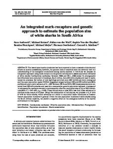
Figure 1. Spectral profiles of the endmembers (a) used to generate the simulated reflectance image (b).

The parameter ρt is not known beforehand. Therefore, an estimate of ρt that serves as a reference to solve (9) is required. The slope of the reflectance spectra at the absorption feature located at 0.944 µm can be reconstructed using spectra value at reference channels by means of interpolation. We used cubic spline interpolation with cross-validation between each pair of adjacent points to set the degree of smoothing. For a simple dataset this is more accurate than other polynomial interpolation methods (Fung 2006). A channel is considered as the reference channel if its signal is not being influenced by any atmospheric species and the signal to noise ratio is large.

4. 4.1.

Datasets Synthetic surface reflectance data

Data are generated following the methodology presented in (Iordache et al. 2012). The reflectance datacube is a hyperspectral image that contains 100 × 100 pixels generated using nine endmembers, namely: leather oak, sandy loam, concrete, dry grass, lime stone, pine wood, red brick, terracotta tiles, and tumble weeds. These endmembers were selected as follows: dry grass and leather oak spectra were obtained from the database of Jasper Ridge, spectral library (ENVI-Team 2014) available in ENVI software (ENVI-Guide 2009) whereas construction, sandy loam, and asphalt spectra were obtained from the database of the Johns Hopkins University Spectral Library (Baldridge et al. 2009). All endmember spectra were resampled to the central wavelengths of the HyMap airborne hyperspectral sensor (Cocks et al. 1998). Hence, the data contain 126 spectral bands (Figure 1a). The simulated data obey the linear mixture model, which satisfies both the sum to one and the non-negativity constrains and are piecewise smooth, i.e., they are smooth with sharp transitions, as shown in Figure 1b. The resulting observations exhibit spatial homogeneity as described in Figure 2, which shows the true abundances of the endmembers. 4.2.

Real Data

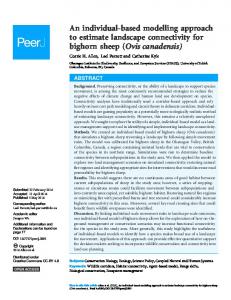
The purpose of using real sensor data is to validate the proposed method and conclusions from the simulated data under real imaging conditions, i.e. with real sensor noise and scene complexity. The scene used here is an Airborne Prism EXperiment (APEX) sensor datacube (2014) over the Liereman area (within 51.30653○ N, 5.013669○ E and 51.33816○ N, 4.984975○ E) in Belgium, shown in Figure 3a. To approximate the size of the simulated image the real scene is cropped into a sub-scene shown in Figure 3b, 6

Figure 2. True fractional abundances of the endmembers in the simulated reflectance image.

at the size of the simulated image (100 × 100). The image of the Liereman area comprises 302 spectral bands between 0.4 µm and 2.5 µm, with a spectral resolution of 4–10 nm depending upon the spectral region. Prior to the analysis, bands contaminated by water absorption and low SNR were removed, leaving a total of 227 spectral bands. Further, it is important to note that this data is cloud free.

5. 5.1.

Experimental Setup Profile of the atmospheric condition parameters for the forward modeling

To transform the synthetic surface reflectance image to at sensor radiance, the atmospheric scattering and absorption conditions must be specified to the MODTRAN 4 radiative code. For this purpose we obtain Aerosol Optical Depth (AOD) and CWV using image based methods (Rodger and Lynch 2001; Richter et al. 2006) applied on a real Airborne Prism EXperiment (APEX) sensor datacube (Schaepman et al. 2015) flight. As an input to these methods, we used three radiance cubes of the Coast of Belgium. The reason for using the coastal area is its diversity, as the scene is covered by both sea and land. These types of scenes are interesting in terms of determining the uncertainty bounds of CWV and AOD for uncertainty exploration as over land and sea these parameters show high variation. This gives us an opportunity to validate the robustness of the proposed methodology for such complexity in the scene. Using the three radiance cubes, for various illumination and viewing geometry, realistic uncertainty estimates of CWV and AOD are obtained. For CWV we obtained a range of 1.35–2.25 g ⋅ cm−2 . Estimating the range of AOD is not straightforward, because the method in (Richter et al. 2006) provides visibility (in km) as an output. In MODTRAN 4, both AOD and visibility are used to describe the aerosol optical properties. In MODTRAN 4, visibility scales the aerosol content in the boundary 7

Figure 3. True color representation of the real APEX RGB image (a) and the sub-scene used in the experiment (b) for the Liereman area, Belgium. The full scene covers 7.5 km2 of area.

layer (0–2 km). Whereas AOD is a pure number specifying extinction due to aerosols at a specific wavelength λ and is the product of the extinction coefficient EXT(λ) and the path length. As visibility tends to increase, the AOD asymptotically decreases. At 550 nm the contributions of molecular depth, ozone depth, trace gases usually are small. Thus, at 550 nm AOD is the main contributor to the total optical depth of the atmosphere i.e. EXT(550) is directly related to the AOD. A high precision in AOD can be achieved by subtracting the Rayleigh scattering coefficient and a very small trace gas depth from a known total optical depth. At 550 nm, visibility is related to AOD by (Berk et al. 2000), visibility =

ln(50) , EXT(550) + 0.01159

(12)

where, 0.01159 km−1 is the surface Rayleigh scattering coefficient at 550 nm. This paper specifically focuses on operational processing chain, where AOD measurements coinciding with image acquisition are often unavailable. Thus, visibility is used to set atmospheric profiles (Schlapfer 1998; Richter et al. 2006; Richter 2007; Biesemans et al. 2007; Sterckx et al. 2016). In MODTRAN 4, visibility is given as a parameter for transmittance simulations for a given illumination and viewing geometry. This leads to a look-up table of visibility against transmittance. Figure 4a shows the relation between visibility and AOD at 550 nm whereas Figure 4b shows atmospheric transmittance at visibility equals 5, 10, 15, and 20 km. Further, determining the range of visibility is challenging because the method in (Richter et al. 2006) is based on the dense dark vegetation (DDV) technique. One of its limitation is that visibility can only be estimated for those pixels. This implies that interpolation is required to estimate visibility for non-DDV pixels. Interpolation methods, however, can induce additional uncertainty in the parameter estimation, requiring a separate analysis. To avoid such uncertainty in further analysis, we first recorded all estimations of visibility for the DDV pixels for the entire scene. We then estimated a marginal density of those visibilities. We used kernel methods to estimate the marginal density of visibility (Silverman 1986). It is implemented using the kde function of the ks package (Duong 2016) in R (R Development Core Team 2008). Parameters, e.g. bandwidth and number of modes, used 8

Figure 4. Relation between visibility and AOD in (a) and effect of visibility on atmospheric transmittance in (b) are shown. Standard MODTRAN 4 Mid-Latitude Summer model with correlated k-option is used while CWV equals 2.0 g ⋅ cm−2 and other atmospheric parameters are at their default values.

Figure 5. Marginal kernel density of visibility estimated using all (≈ 80 thousand) measurements from the image based method. A bandwidth of 1.56 is used as a parameter for kernel density estimation.

to estimate the marginal densities, are obtained from the h.crit and nr.modes functions as illustrated in the silvermantest package in R (Silverman 1981; Hall and York 2001). In Figure 5 the estimated marginal density of visibility is shown. From the marginal density, we observe a skewed distribution which covers the range between 15 and 120 km. From our experience with the optical parameters in the CDPC, we realized that visibility >60 km has little impact on the estimate of reflectance. Thus, we limit the possible range of visibility to 15 to 65 km, which is approximately equivalent to the AOD range 0.47–0.13. To simulate the average background radiance for the forward modeling i.e. for the adjacency effect, average radiance of the surrounding pixels should be incorporated. The average radiance is a function of: 1) the extent of neighborhood r of pixels that can spatially influence the target pixel and 2) a weight function within the background window to obtain average radiance. We distinguish two factors that influence calculation of r and weights within the r × r neighborhood: scattering conditions and spatial cross correlation. In (Tanre et al. 1987), an environmental function is proposed that determines r and assigns weights to neighborhood pixels based upon the scattering condition. An implementation of this method can be found in (Sterckx et al. 2011). In this work we refrain from such 9

calculations as our experiments with the real images in the CDPC (Bhatia et al. 2015) showed that for a strong water absorption feature of 944 nm the scattering effect is insignificant. Following (Richter 2007), we use range dependent function with an exponential decrease to assign weights to the neighborhood pixels. The minimum value of r is determined through a variogram analysis whereas the maximum value of the r was set to 91 pixels. This limit was enforced by the spatial extent of the simulated and the real sub-image (100 × 100 pixels). To obtain the variogram for the simulated dataset and for the real dataset we used the function vgram.matrix of fields package in R. 5.2.

Pixelwise parameter configuration for the forward modelling

From the ranges of visibility, CWV, and r, we now derive their spatial pattern or variability over each pixel as we may and in real scenes for the forward modeling. For the simulated dataset, we assumed a gradual increase in CWV as we move row wise from the top of the simulated dataset to the bottom. We assigned a value CWV = 1.35 g ⋅ cm−2 to the central pixel of the first row. The other pixels of this row received randomly sampled values from the N (1.35, 0.02) distribution. Likewise, with a step of 0.00912 g ⋅ cm−2 we assigned values to pixels of each row. The resultant spatial variability of CWV is shown in Figure 6a.

Figure 6. Spatial variability of CWV in (a), visibility in (b), and background window in (c) of the simulated image.

A similar procedure was applied to visibility which varies between 15 km and 65 km corresponding to an AOD range 0.47–0.13. The direction of variation is taken from the left of the simulated image to the right, i.e. column wise, with a step size of 2 km. To each pixel in a column, randomly sampled values from the log N (µ, 0.02) with µ = 15 km for the first column are assigned. A log-normal distribution is used to approximate the actual distribution of visibility, being a skewed normal distribution (Figure 5). For the adjacency effect, we considered the spatial variability of the classes present in the simulated image. From visual interpretation we found it spectrally more homogeneous at the center of the image than at the edges. Moving away from the center of the image, this homogeneity weakens (Figure 1b). As spectrally homogeneous pixels cause a low adjacency effect, a significant influence on the center pixels can only come from pixels that are far away from the center. To address this spatial variability we set a large r = 91 pixels at the center of the image. The range gradually decreases as we move away from the center of the image and to a minimum of 41 pixels (Figure 6c). This value was determined from the variogram analysis.

10

5.3.

Addition of noise in both the datasets

Sensor noise and processing noise are major sources of distortion of the images. Sensor noise refers to the random electronic noise like dark current, whereas processing noise refers to the spectral smoothing applied on a reflectance datacube in a final preprocessing step, introducing correlated noise. We thus added noise to the simulated datacube at two stages: white noise (random noise) to the radiance cube, at sensor level and correlated noise to the estimated reflectance cube. As the real dataset is already contaminated with sensor noise, we only added correlated noise. To observe the effect of different noise levels we considered correlated noise at three signal-to-noise ratios (SNR): 30, 40, and 50 dB, respectively. All correlated noise levels were generated from independent, identically distributed i.i.d. Gaussian (white) noise by low pass filtering with a normalized cut off frequency of 8π B for each SNR. For the simulated dataset, adding random noise is challenging. The reason is that from our experience with images processed in the CDPC, we observed that noise with a specific SNR added at sensor level can more severely damage the data as compared to the same noise added at the reflectance level. Thus, we added white noise with SN R = 60 dB to the simulated radiance datacube and correlated noise with SNR ranging from 30 to 50 dB to the estimated reflectance cubes. These SNR levels are lower than the specified range of the APEX sensor (Schaepman et al. 2015). This implies that we are testing at higher noise levels than the specified conditions. 5.4.

Performance Discriminators

The quantitative assessment of the propagation of uncertainty originating from the AC E [∥x∥22 ] , where parameters is measured by the signal-to-reconstruction-error SRE ≡ E [∥x−x ˆ∥22 ] x is the reference signal and x ˆ represents its estimation. SRE provides information on the power of the signal with respect to the power of the error (Iordache et al. 2011). In all experiments, we report SRE measured in dB: SRE(dB ) = 10log10 (SRE). Together with the SRE, we also measured the Root Mean Squared Error (RMSE) of the estimated and reference data.

6. 6.1.

Experimental Results Experiments with simulated data

We first present the estimation results for CWV without considering noise, visibility, and adjacency. To achieve this, reference values of visibility and adjacency are used for each pixel (Figure 6b and Figure 6c). First, the CWV is set equal to 1.6 g ⋅ cm−2 . At those pixels where this value is used in forward modeling, reflectance estimation at absorption features leads to a correct estimate (Figure 6a). For other pixels, CWV = 1.6 g ⋅ cm−2 will either underestimate or overestimate the reflectance at water absorption features, depending upon whether it is smaller or larger than the value used in forward modeling. In Figure 7 a spectral plot of the class concrete from three different image regions is depicting correct, over-, and under-estimation scenarios. The pixel wise coefficient values indicate correct estimation, overestimation, and un11

Figure 7. Overestimation (◻), underestimation ( ), and correction estimation (△) of reflectance for pixels where the class concrete dominates the initial water vapor value (1.6 g ⋅ cm−2 ).

derestimation of reflectance at absorption features as shown in Figure 8a. We observe coefficient values close to 1 at those pixels for which 1.6 g ⋅ cm−2 is used in forward modeling i.e. the correct estimation of reflectance at the absorption feature. The robustness of our method can be observed in Figure 8b where small or no changes in CWV values are observed if their corresponding coefficients are close to one. For the other pixels, CWV values lower and higher than 1.6 g ⋅ cm−2 are set for which the reflectance is over- or under-estimated, respectively.

Figure 8. Pixel wise coefficient values at 0.944 µm (a), new estimates of CWV for each pixel (b), absolute difference between the new and previous estimations of CWV (c), and absolute difference between the new and reference CWV values (d) obtained after the first iteration.

From Figure 8c–d we observe small absolute errors between the previous and new CWV values, and between the new and reference CWV values if the reflectance is approximately correctly estimated. We observe large absolute errors if the reflectance is either over- or under-estimated. Iteratively estimating the CWV, we observe that the coefficients for each pixel are approaching one and that errors tend to be small. This is confirmed from Figure 9a–d, showing the CWV after 15 iterations. 12

Figure 9. Pixel wise coefficient values at 0.944 µm (a), new estimates of CWV over each pixel (b), absolute difference between the new and previous estimations of CWV (c), and absolute difference between the new and reference CWV values (d) obtained after 15 iterations.

Figure 10. SRE (dB) and RMSE obtained during CWV estimation at successive iterations.

Estimates converged after 20 iterations, as can be seen in Figure 10. As is evident from these, CWV estimation improved after each iteration. This implies that the solution is leading towards convergence. We already observed convergence after the 15th iteration, followed by small improvements for higher iterations. Figure 11 presents the impact of CWV estimates on the reflectance estimation. We observe convergence of estimation of reflectance after 10 iterations. Continuing CWV estimation for 12 iterations did not result in any further improvement. The objective of the second experiment was to include noise to the data and to perturb the spatial variability of visibility and adjacency while estimating CWV. This scenario is similar to real imaging conditions. We applied rotation to the reference values of visibility and the background window size defined for each pixel (Figure 6b and Figure 6c). We also applied spatial smoothing to the visibility values at each pixel after the rotation (Figure 13) and measured visibility and background window with diagonal spatial variability Figure 14–16. The reason to rotate and smooth the reference data and to realize diagonal variability, is to realize different ways to arrange visibility and adjacency in the spatial domain.

13

Figure 11. SRE (dB) and RMSE computed for CWV estimates at reflectance level for each iteration.

Figure 12. Coefficients values for CWV estimation after 10 iterations.

From Figure 17, we observe that noise and the arbitrary setting of visibility and the background window do not influence the estimation of CWV. This experiment showed that the method presented in this paper estimates CWV correctly if no prior information about the CWV is present, using an arbitrary value of 1.6 g ⋅ cm−2 for CWV to start the estimation. 6.2.

A comparison study

For performance assessment, we compared the new method with two state-of-the-art methods. Method 1 (M1 ) (Rodger and Lynch 2001) is currently implemented in the CDPC and it estimates CWV using at sensor radiance. Method 2 (M2 ) (Rodger 2011) uses variations of a second order derivative algorithm (SODA) to assess the impact of atmospheric residual features on calculated surface reflectance spectra after AC. Performance is assessed in two ways. First, computational efficiency of the methods is compared with the proposed method, which is critical in operational processing chains. Second, the accuracy of each method is measured in terms of the absolute error. M1 estimates CWV in five steps. In each step it generates a number of synthetic at sensor spectral signals each with a different amount of atmospheric CWV. After applying scaling to the signals and to the actual at sensor radiance, it iteratively determines CWV values. These steps are repeated until convergence is reached. Applying 14

Figure 13. Pixel wise perturbation to the spatial variability of visibility with (a) 90○ rotation, (b) no rotation, (c) 180○ rotation, and (d) 270○ rotation.

Figure 14. Pixel wise perturbation to the spatial variability of visibility with diagonal variation (a) top left to bottom right, (b) bottom left to top right, (c) bottom right to top left, (d) top right to bottom left.

M1 on the synthetic image, results in convergence in 5–6 iterations. The accuracy in terms of absolute error is shown in Figure 18 where the maximum absolute error equal to 0.42. This is a large value as compared to 0.015 of the proposed model (Figure 19). Method 2 calculates the surface reflectance multiple times using several CWV values to obtain a complete set of SODA values corresponding to the N surface reflectance values. This set is searched for the value that yields the lowest SODA, which is assumed to be the true value of the reflectance. Its corresponding CWV value is the estimated value. The minimum recommended value of N for M2 is 50, e.g. M2 estimates CWV 15

Figure 15. Pixel wise perturbation to spatial variability of the background window with no rotation (a) and 90○ rotation (b).

Figure 16. Pixel wise perturbation to the spatial variability of the background window with diagonal variation (a) top left to bottom right, (b) bottom left to top right, (c) bottom right to top left, (d) top right to bottom left.

Figure 17. SRE (dB) and RMSE values obtained during CWV estimation for successive iterations with noise applied to the data and visibility and background window incorrectly set.

with at least 50 iterations. The proposed method, however, requires 8–10 iterations for pixelwise estimate of CWV with the absolute error minimized close to zero. Iteration times of M2 and the proposed method are comparable because both use MODTRAN 4 to estimate various radiance components for AC (7). Also, M2 first estimates CWV for a super pixel and in a later stage only it calculates pixelwise CWV. This leads to additional computational time that is critical within a processing chain.

16

Figure 18. Pixel wise estimation of CWV using the method described in (Rodger and Lynch 2001) (a) and in (b) the absolute error between the prior estimates of CWV in (a) and the reference CWV is shown.

Figure 19. Pixel wise coefficient values at 0.944 µm (a), new estimates of CWV for each pixel (b), absolute difference between the new and previous estimations of CWV (c), and absolute difference between the new and reference CWV values (d) obtained after the 8th iteration.

6.3.

Calibration of CWV

To analyze the performance of the proposed method while calibrating CWV, we first applied the method described in (Rodger and Lynch 2001) to obtain initial estimate on CWV, shown in Figure 18. We then used these pre-estimates to our method. In Figure 19, CWV values are shown after 8 iterations. We observe that the proposed method successfully calibrates CWV. An important observation during calibration and CWV estimation is that small improvements in CWV estimation do not further improve reflectance estimation after a relatively low number of iterations. The acceptable degree of change, i.e. the tolerance limit, is quantified by assessing the coefficients values at the 10th iteration (Figure 12). The CWV coefficients range between 0.9765 and 1.045. Using (10), we obtained a range of 0.0235–0.045 g ⋅ cm−2 , specifying the tolerance limit in CWV estimation at the reflectance level. 6.4.

Experiments for the real scene

For the real scene (Figure 3b), the range for CWV is between 1.5 and 2.4 g ⋅ cm−2 . To check robustness of the proposed method, we selected at random CWV values within a narrow range of 1.5–1.6 g ⋅ cm−2 for the first iteration. This pixelwise assignment 17

Figure 20. Absence of spatial variability of CWV for each pixel during the first iteration.

Figure 21. SRE (dB) and RMSE values using reference coefficients and estimated fitting coefficients obtained after seven iterations.

avoids any prior knowledge about the scene. In Figure 20, the CWV values at each pixel are shown. For the real scene, reference data are not available. Thus, to validate the results we computed SRE (dB) and the RMSE at coefficient level for each pixel. The resultant performance plot is shown in Figure 21. From Figure 21, we observe that our method works well for the real dataset, as perceived from the coefficient’s SRE and RMSE values. Also, we observe that the coefficients can be further improved i.e. estimation of CWV can be improved with more iterations. Performing seven iterations was sufficient, as applying more iterations show no substantial improvement in the coefficients values.

7.

Discussion and Conclusion

This paper presents a method that iteratively estimates CWV from reflectance spectra. It was applied to two hyperspectral sensors and there is no reason why it should also not be effective on other hyperspectral sensors. The method is simple to implement and can be extended to encompass other atmospheric trace gases. Its main benefit is that it is free from any assumptions that are usually made for at sensor radiance based CWV estimation methods. For instance, it does not require the surface reflectance to be linear across spectral absorption features, nor does the spectral reflectance require pre-smoothing. A water profile obtained using the first assumption is only applicable 18

to scenes that show a linear surface behavior across different wavelengths. Such a linearity assumption is not valid for a reflectance spectrum of a complex and variable surface. The study further shows that the method works well under noisy conditions, i.e. if the second assumption does not hold. With the proposed method, noise and incorrect estimation of AOD and the background window have little to no influence on CWV estimation. The reason is that these perturbations affect the amplitude of the spectra of a pixel and do not contribute to over- and underestimation of reflectance at the absorption feature. These findings are, however, only valid for high visibility values (> 18 km). Under lower visibility conditions the effect of AOD on CWV retrieval is significant (Chylek et al. 2003) and might have influenced the retrievals. Airborne campaigns, however, occur on clear days, that is when visibility is sufficiently high. This is for example evident from the visibility range observed for the real scene. These findings, well-known from the literature, were helpful in validating our method. Thus, for strong water absorption features, the quality of CWV estimation is dominant over visibility, the adjacency effect and noise correlation. Also, for higher visibility values (>18 km), estimation of CWV can be performed without setting visibility and the background window to their actual values. This is consistent with our previous work (Bhatia et al. 2015) in which we found that CWV is the most important parameter at strong absorption features. We further observed that our method works well when calibrating the prior CWV estimates from the in-built method to estimate CWV. From theoretical considerations this is what we might expect assuming that our method works well if prior estimates are available. We found that the number of iterations required for calibration is less as compared those needed for CWV estimation. For at sensor based CWV estimation, influences of sensor noise and uncertainty arising from instrument characterization are generally estimated in a laboratory prior to flight. Such estimation requires linearity of the detectors, gains and offset of the sensor, and spectral response of the sensor channels. If any of the above assumptions is not fulfilled, then the estimated CWV contains residual effects in the absorption features. Such effects cause the relation between CWV and the absorption feature to become non-linear. Due to non-linearity, an absorption feature cannot be related with CWV, as otherwise it will be prone to errors. In contrast to at sensor based estimation of CWV, our method does not require a separate modeling to account for errors induced due to other influencing factors. Estimating CWV based on reflectance spectra results into a linear relation between residuals at absorption features and CWV. This is because reflectance spectra are obtained after atmospheric corrections. It implies that all errors are already modeled and show their effects as over- or under-estimation at an absorption feature. The pivot of the methodological choices in this paper is its use in an operational chain. From this point of view we note that the processing time to estimate CWV is low. In particular, the number of iterations to pixel wise estimate CWV is between 8 and 10. The reason why we could estimate CWV with less iterations is because for each iteration the new estimates are fed back into atmospheric correction procedures. This is different from estimation based upon reflectance spectra for a set of CWV values, followed by value optimization. See e.g. the SODA method described in (Rodger 2011). Also, solving CWV for each pixel for a set of CWV values in an operational chain environment requires a much higher computing time.

19

References Baldridge, A. M., S. J. Hook, C. I. Grove, and G. Rivera (2009). The aster spectral library version 2.0. Remote Sensing of Environment 113 (4), 711 – 715. Berk, A., G. P. Anderson, P. K. Acharya, J. H. Chetwynd, L. S. Bernstein, E. P. Shettle, M. W. Matthew, and S. M. Adler-Golden (2000). MODTRAN4 user’s Manual. Technical report, Air Force Research Laboratory, Hanscom AFB, MA, USA and Naval Research Laboratory, Washington, DC, USA and Spectral Sciences, Burlington, MA, USA. Bhatia, N., V. A. Tolpekin, I. Reusen, S. Sterckx, J. Biesemans, and A. Stein (2015). Sensitivity of Reflectance to Water Vapor and Aerosol Optical Thickness. IEEE Journal of Selected Topics in Applied Earth Observations and Remote Sensing 8 (6), 3199–3208. Biesemans, J., S. Sterckx, E. Knaeps, K. Vreys, S. Adriaensen, J. Hooyberghs, K. Meuleman, P. Kempeneers, B. Deronde, J. Everaerts, D. Schlapfer, and J. Nieke (2007, April). Image processing work flows for airborne remote sensing. In Proceedings 5th EARSeL Workshop on Imaging Spectroscopy. European Association of Remote Sensing Laboratories (EARSeL). Burazerovic, D., R. Heylen, B. Geens, S. Sterckx, and P. Scheunders (2013). Detecting the Adjacency Effect in Hyperspectral Imagery With Spectral Unmixing Techniques. IEEE Journal of Selected Topics in Applied Earth Observations and Remote Sensing 6 (3), 1070– 1078. Carrere, V. and J. Conel (1993). Recovery of atmospheric water vapor total column abundance from imaging spectrometer data around 940 nm – sensitivity analysis and application to airborne visible/infrared imaging spectrometer (aviris) data. Remote Sensing of Environment 44 (2), 179–204. Chylek, P., C. C. Borel, W. Clodius, P. A. Pope, and A. P. Rodger (2003, Dec). Satellitebased columnar water vapor retrieval with the multi-spectral thermal imager (mti). IEEE Transactions on Geoscience and Remote Sensing 41 (12), 2767–2770. Cocks, T., T. Jenssen, A. Stewart, I. Wilson, and T. Shields (1998, October). The hymaptm airborne hyperspectral sensor: The system, calibration and performance. In In Proceedings of the 1st EARSeL Workshop on Imaging Spectroscopy, Zurich, pp. 37–42. European Association of Remote Sensing Laboratories (EARSeL). Duong, T. (2016). ks: Kernel Smoothing. R package version 1.10.3. ENVI-Guide (2009). ”ENVI EX Users Guide”,. Technical report, ITT Visual Information Solutions. ENVI-Team (2014). ENVI Classic Tutorial: Vegetation Hyperspectral Analysis. Technical report, Exelis Visual Information Solutions, Inc. Fung, D. S. (2006). Methods for the estimation of missing values in time series. Master’s thesis, School Of Mathematics and Engineering, Edith Cowan University, Perth. Gao, B. C., C. Davis, and A. Goetz (2006, July). A review of atmospheric correction techniques for hyperspectral remote sensing of land surfaces and ocean color. In 2006 IEEE International Symposium on Geoscience and Remote Sensing, pp. 1979–1981. Gao, B. C., M. J. Montes, C. O. Davis, and F. H. Goetz, A. (2009). Atmospheric correction algorithms for hyperspectral remote sensing data of land and ocean. Remote Sensing of Environment 113, S17 – S24. Imaging Spectroscopy Special Issue. Gao, B. G. and A. F. H. Goetz (1990). Column atmospheric water vapor and vegetation liquid water retrievals from airborne imaging spectrometer data. Journal of Geophysical Research: Atmospheres 95(D4), 3549–3564. Gao, B., C. and Y. J. Kaufman (2003). Water vapor retrievals using moderate resolution imaging spectroradiometer (modis) near-infrared channels. Journal of Geophysical Research: Atmospheres 108(D13). Haan, J. F. and J. M. M. Kokke (1996). Remote sensing algorithm development Toolkit I: Operationalization of atmospheric correction methods for tidal and inland waters. Development Toolkit NRSP-2 96-16, Netherlands Remote Sensing Board. Hall, P. and M. York (2001). On the calibration of Silvermans test for multimodality. Statistica Sinica 11, 515–536.

20

Iordache, M. D., J. M. Bioucas-Dias, and A. Plaza (2011). Sparse Unmixing of Hyperspectral Data. IEEE Transactions on Geoscience and Remote Sensing 49 (6), 2014–2039. Iordache, M. D., J. M. Bioucas-Dias, and A. Plaza (2012). Total Variation Spatial Regularization for Sparse Hyperspectral Unmixing. IEEE Transactions on Geoscience and Remote Sensing 50 (11), 484–4502. Kaufman, Y. J. and C. Gao, B. (1992). Remote sensing of water vapor in the near ir from eos/modis. IEEE Transactions on Geoscience and Remote Sensing 30 (5), 871–884. Qu, Z., B. C. Kindel, and A. F. H. Goetz (2003, June). The high accuracy atmospheric correction for hyperspectral data (hatch) model. IEEE Transactions on Geoscience and Remote Sensing 41 (6), 1223–1231. R Development Core Team (2008). R: A Language and Environment for Statistical Computing. Vienna, Austria: R Foundation for Statistical Computing. Richter, R. (2007). Atmospheric/Topographic Correction for Airborne Imagery (ATCOR-4 User Guide). User guide, DLR-German Aerospace Center. Richter, R., D. Schlapfer, and A. Muller (2006). An automatic atmospheric correction algorithm for visible/NIR imagery. International Journal of Remote Sensing 27 (10), 2077–2085. Rodger, A. (2011). Soda: A new method of in-scene atmospheric water vapor estimation and post-flight spectral recalibration for hyperspectral sensors: Application to the hymap sensor at two locations. Remote Sensing of Environment 115 (2), 536–547. Rodger, A. and J. M. Lynch (2001, 27th February – 02 March). Determining Atmospheric Column Water Vapour in the 0.4- 2.5 m spectral region. In Proceedings of the AVIRIS Workshop Pasadena, California. Jet Propulsion Laboratory (JPL) publication, USA. Schaepman, M. E., M. Jehle, A. Hueni, P. D’Odorico, A. Damm, J. Weyermann, F. D. Schneider, V. Laurent, C. Popp, F. C. Seidel, K. Lenhard, P. Gege, C. Khler, J. Brazile, P. Kohler, L. D. Vos, K. Meuleman, R. Meynart, D. Schlapfer, M. Kneubhler, and K. I. Itten (2015). Advanced radiometry measurements and Earth science applications with the Airborne Prism Experiment (APEX). Remote Sensing of Environment 158, 207–219. Schaepman, M. E., M. Jehle, A. Hueni, P. D’Odorico, A. Damm, J. Weyermann, F. D. Schneider, V. Laurent, C. Popp, f. C. Seidel, K. Lenhard, P. Gege, C. Kuchler, J. Brazile, P. Kohler, L. D. Vos, M. Meuleman, R. Meynart, D. Schlapfer, M. Kneubuhler, and K. Itten (2015). Advanced radiometry measurements and earth science applications with the airborne prism experiment (apex). Remote Sensing of Environment 158, 207 – 219. Schlapfer, D. (1998). Differential Absorption Methodology for Imaging Spectroscopy of Atmospheric Water Vapor. Ph. D. thesis, Remote Sensing Laboratories, Department of Geography, Universiy of Zurich. Silverman, B. W. (1981). Using Kernel Density Estimates to investigate multimodality. Journal of the Royal Statistical Society 43 (1), 97–99. Silverman, B. W. (1986). Density Estimation for Statistics and Data Analysis. London: Chapman and Hall/CRC. Staenz, K., J. Secker, C. Gao, B., C. Davis, and C. Nadeau (2002). Radiative transfer codes applied to hyperspectral data for the retrieval of surface reflectance. {ISPRS} Journal of Photogrammetry and Remote Sensing 57 (3), 194 – 203. Stamnes, K., S.-C. Tsay, W. Wiscombe, and K. Jayaweera (1988, June). Numerically stable algorithm for discrete-ordinate-method radiative transfer in multiple scattering and emitting layered media. Applied Optics 27 (12), 2502–2509. Sterckx, S., E. Knaeps, and K. Ruddick (2011). Detection and correction of adjacency effects in hyperspectral airborne data of coastal and inland waters: the use of the near infrared similarity spectrum. International Journal of Remote Sensing 32 (21), 6479–6505. Sterckx, S., K. Vreys, J. Biesemans, M. D. Iordache, L. Bertels, and K. Meuleman (2016). Atmospheric correction of APEX hyperspectral data. Miscellanea Geographica Regional Studies Development 20 (1). Tanre, D., P. Y. Deschamps, P. Duhaut, and M. Herman (1987). Adjacency effect produced by the atmospheric scattering in thematic mapper data. Journal of Geophysical Research: Atmospheres 92 (D10), 12000–12006.

21

Verhoef, V. and H. Bach (2003). Simulation of hyperspectral and directional radiance images using coupled biophysical and atmospheric radiative transfer models. Remote Sensing of Environment 87 (1), 23 – 41. Verhoef, W. (1998). Theory of radiative transfer models applied in optical remote sensing of vegetation canopies. Ph. D. thesis, University of Wageningen, Netherlands.

22