recommend using metrics during the test phase of software development and propose additional candidate metrics ...... Reporting such data can become part of the overall computer system manager's accounting activities .... Itemized DR List:.
AN EVALUATION OF SOFTWARE TESTING METRICS FOR NASA'S MISSION CONTROL CENTER George E. Stark, Robert C. Durst, Tammy M. Pelnik The MITRE Corporation Houston, TX Abstract Software metrics are used to evaluate the software development process and the quality of the resulting product. We used five metrics during the testing phase of the Shuttle Mission Control Center (MCC) Upgrade (MCCU) at the National Aeronautics and Space Administration's (NASA) Johnson Space Center. All but one metric provided useful information. Based on our experience we recommend using metrics during the test phase of software development and propose additional candidate metrics for further study. Introduction Testing is the process of executing a program with the intention of finding faults.1 Software project managers evaluate the testing progress and take corrective actions, if necessary, on risk (which subsystems are likely to delay progress?), quality (how many complaints can I expect from the user community each year?), cost allocation (how much should I budget for maintenance?), and schedule (how close am I to being finished?). Managers traditionally have evaluated test progress using programmer and test team intuition, percentage of tests completed, and/or successful execution of critical functional tests. Intuition is notoriously bad since people are usually optimistic about their progress. Percentage of tests complete gives no indication of the operational impact of the tests not yet completed. The critical functional test method gives a limited view of software status, but gives no indication of the expected number of failures in operation. The weaknesses of these traditional approaches have led to the development of software metrics. Software metrics aid evaluation of the testing process and the software product by providing objective criteria and measurements for management decision-making. In this paper we evaluate the applicability of five software metrics (Software Size, Software Reliability, Test Session Efficiency, Test Focus, and Software Maturity) based on our experience during the test phase of NASA's MCCU project. We briefly describe the MCCU environment and the collected data. We then define each metric, discuss our experience with it, and provide a set of lessons learned. Finally, we describe additional metrics that merit further investigation. The MCCU Environment The MCCU project was initiated in the mid-1980s to address key architectural and operational goals in the MCC: replacing aging equipment, reducing reconfiguration time, and improving operator usability of the system (thereby reducing requisite training time). The MCCU project introduces a distributed computing environment into the MCC. The environment contains UNIX workstations and associated data drivers connected by Local Area Networks (LAN) to centralized host computers.
The MCCU is being implemented in phases and delivered incrementally within each phase. Delivery 2.5 contains the bulk of the distributed environment and its supporting software. The upgrade has resulted in new operating procedures (and associated software systems) for the workstations while the host processing has remained relatively stable. Kearney2 provides a complete description of the MCCU goals and architecture. The software consists of twenty-five subsystems containing over 800,000 executable source lines of code distributed across the key MCCU components as shown in Table 1. Component Hosts Local Area Networks Workstations Data Drivers Total
Source Lines of Code 131,204 162,382 365,776 156,000 815,362
Table 1. Delivery 2.5 Source Lines of Code by Component Eighteen percent of the code is assembly language; 82% is written in ‘C’. Metrics gathered during the testing phases of Delivery 2.5 are the subject of this paper. The MCCU Delivery 2.5 software was developed over a two-year period distributed as follows: eight months from System Design Review to software Critical Design Review (CDR), six months from CDR to Start of Test Review (STR), and ten months from STR to Final Acceptance Review (FAR). The six-month period from CDR to STR contained the coding, unit testing, and subsystem qualification testing phases, which were conducted at the contractor facilities. Successful completion of these testing phases is the criteria for entry into integration verification testing. This study is solely limited to the ten-month time frame from STR to FAR. This period contained four development test phases: (1) Integration Verification Test: Requirements-oriented testing in a system environment (i.e., all available software/hardware components have been combined). Tests are detailed interface tests among various subsystems examining system timing, performance, and high-level functionality. (2) System Delivery Test: Testing that exercises functionality in a simulated operational configuration and work environment. (3) Stress Test: Verification of the overall functionality and system limitations under extreme load conditions (extremes in transactions/minute, data rate, displays, etc.). (4) Final Acceptance Test: User-performed testing to certify that the delivered product performs to requirements, does not degrade existing capabilities, and meets operational flight support needs. Because the MCC is an operational facility, a number of activities compete for its resources: mission support, flight controller training, reconfiguration, preventive maintenance, and development testing. Development testing has the lowest priority of these activities. Thus, the total of 1150 active
2
test hours for Delivery 2.5 were not uniformly distributed over the calendar time period. Figure 1 is a plot of the active test hour distribution by month and test phase for the period under study. Note that since the test hours are not equally distributed, data normalization by day or month would lead to erroneous conclusions.
250 200 Active 150 Test Hours 100
1
2
3
4
50 0
0
2
4
STR
6 Month
8
10
12
FAR
1 Integration and Verification Test 2 System Delivery Test 3 Stress Test 4 Final Acceptance Test Figure 1. Active Test Hours by Phase and Month Collected Data The metric definition and analysis was constrained to use available data in order to avoid perturbing the ongoing development process. This section describes the basic data available and the quality of that data. The study period consisted of 126 test sessions. At the end of each test session, a test session report form was completed by the test monitor. A sample test session report form is shown in the appendix. In general, the form required the test monitor to answer several short questions; answers document the impact of all observed failures and other characteristics of the test session. The following information from the form was used to calculate and evaluate the metrics: (1) Discrepancy Report count, impact, and subsystem charged (2) Scheduled test time
3
(3) Effective test time (4) Test session rating During each test session the individual testers complete a form describing each failure occurrence. The form is called discrepancy report (DR). A completed DR form contains details of the test environment and the behavior of the system when the failure occurred. All DRs are classified by their failure impact as either critical, major, or minor. At the conclusion of each test session all DR forms are delivered to the development organization for investigation and resolution. Not all DRs indicate software failures. As each DR is closed, the method of closure is also recorded as either (1) closed with a software fix or (2) closed without a software fix. There are several reasons for a DR to be closed without a software fix: requirements change, hardware or operator failure, duplicate DR, etc. DRs closed with a software fix indicate that a fault was identified, corrected, and tested. The quality of the test session data was checked via independent inspection. Occasionally, an anomaly or contradiction arose through the inspection or subsequent analysis. If the data reporting was inconsistent across testers, the test monitor who filed the report was interviewed for clarification. For example, some testers did not fill out a DR form if a subsystem other than the one under test failed during the session. Fortunately, this data could be inferred from the summary text on the test session report form, usually in the form's "Highlights" or "Lost Time" sections. An example of such an inference is the determination of the number of failures during a test session. Since a description read "host crashed and we lost x hours while the offending subsystem's development team investigated," but no DR form was completed since the tester was "not testing the host," a failure could be inferred with reasonable certainty. Data was not incorporated into the data set used for this analysis if the inference was deemed unreliable.
Description of Analyzed Metrics The MCCU had some metrics in place prior to this effort (e.g., percent of test cases complete, requested and scheduled test hours, and total DRs by week). To provide additional visibility we used the available data and defined the following set. Software Size Software size, is measured by a count of the source lines of code (SLOC). A source line of code is counted as any line of program text that is not a comment or blank line, regardless of the number of statements or fragments of statements on the line. It reflects all SLOC in the system, not just those currently in test. The goal of this metric is to show the risks to the system over time. Large increases in software size late in the development cycle often result in increased testing and maintenance activities. Thus, if an increase above some pre-determined threshold occurs, management should take corrective action. As a general rule of thumb, changes within a reporting period should be within a 5% range3, assuming at least six reporting periods within the test phase. Whenever the rule of thumb is violated, any of the following actions may be advisable:
4
(1) Account for the change in both the schedule and the project staffing (2) Review test plans and procedures to ensure that the change is covered in the existing plans (3) Evaluate system computer resource impact to ensure that adequate resources will be available (4) Evaluate the impact on sustaining engineering, modifying plans as necessary Software Reliability Software Reliability is the probability of failure-free operation of a computer program for a specified time in a specified environment. Musa4 has defined four uses for the software reliability metric. Our goal for the metric is to quantify the progress of the product toward a specified quality objective.** More than forty models have been proposed in the literature5 for the estimation of software reliability based on data gathered during the test phase. The Musa basic execution time model6 was used during the MCC test phase because (1) it has been widely applied and studied7,8,9; (2) the model assumptions are simple and satisfied in our environment; and (3) there are automated tools available to calculate model parameters10. There are several key assumptions to the Musa model.5 (1) Failures† of the system are caused by faults in the software. Faults are independent and are distributed in the software with a constant average occurrence rate between failures. (2) Execution time between failures is large compared to average instruction execution time. (3) Testing represents the actual operating environment of the software. (4) All failures that occur are detected. (5) The fault that causes each failure is removed with certainty (i.e., failures caused by the same fault are not counted). Using these assumptions, the instantaneous failure rate, z(t), becomes z(t) = (h)exp(-ht/N)
(1)
where N is the number of faults inherent in the program prior to the start of testing, and h is the failure rate prior to the start of testing. Equation (1) is also known as the hazard rate. It provides the theoretical basis for fitting an exponential curve to the empirical failure rate data. It is a particularly useful equation for two reasons: first, it is readily interpretable as the tendency of the software to fail as a function of elapsed time (e.g., 1 failure every 7 hours), and second, all salient functions of the elapsed time to fail of the system can be derived from it, including the probability density and reliability functions. A graph of equation (1) is shown in figure 2. The decreasing failure rate of equation (1) represents "growth" in the reliability of software as
** An objective can be specified by minimizing life-cycle cost11, by balancing the hardware, software, and human failure expectations12, or by working backwards from a required release date6. † We use the IEEE Standard 729 definitions that a failure is the departure of the system from operational requirements, a fault is an internal problem with the code, and an error is the programmmer omission or commission that caused the fault.
5
testing and debugging continue. The reliability of software is expressed as u R(u) = exp(- ⌠ ⌡z(x)dx ) = exp(-uz(x)) = exp(-u/MTTF). (2) Here u is the projected execution time in the future, and x is a variable of integration. The MTTF is the mean time to failure of the software (i.e., the average active time until a failure occurrence). MTTF is calculated as MTTF = (1/h)exp(ht/N) = 1/z(t).
(3)
Possible corrective actions include increasing user test planning involvement, increasing user training, replanning subsystem integration, or reallocating schedules, staffing plans, and resources to account for further testing.
Failures per Hour
Current failure rate
Failure rate objective Remaining Test Time Time Figure 2. A Graph of Instantaneous Failure Rate Test Session Efficiency The goal of the test session efficiency metric is to identify trends in the scheduled test time's effectiveness (i.e., the percent of scheduled test time that is productively used). If facility resources are limited, planning will be more realistic given an understanding of how efficiently the scheduled test time is used. The metric is based on scheduled and active times from each test session report and tester's perception of the effectiveness of the test session. The System Efficiency (SYSE) is calculated as
6
SYSE = (Active test time)/(Scheduled test time)
(4)
for each session for each computer type (workstation or host). At the end of each session, testers are asked to evaluate the session on a binary scale (Good or Bad). The tester efficiency (TE) is then calculated as TE = (Number of good runs)/(Total runs).
(5)
TE is subjective but provides an indication of how well the test personnel believe they are doing. SYSE identifies how much time is spent doing non-testing activities (e.g., set-up/tear-down, DR writing, etc.). As a rule of thumb, both SYSE and TE should be greater than 80%. If the values are significantly below this threshold management should review the test environment, tester preparation, and test procedures. In general, dips in testers' perceptions should correlate to dips in SYSE; when these two items do not correlate, corrective action may be necessary. Possible corrective actions include scheduling more test time, changing the test order, or reallocating time to areas that need it most. Test Focus The goal of the test focus (TF) metric is to identify the amount of effort spent finding and fixing "real" faults versus the effort spent either eliminating "false" defects or waiting for a hardware fix. It is the ratio TF = (Number of DRs closed with a software fix). (Total number of DRs)
(6)
TF provides insight into whether test effort is spent finding and fixing faults in the software, or finding and fixing problems in the test system. An implicit assumption in the extrapolation of the metric value to effort is that the time to discover a problem is relatively constant regardless of whether the fault is in software, hardware, or procedures. The goal of the testing process is to identify errors in the software under test. Therefore, in an ideal case TF approaches unity (that is, all errors found were software errors and resulted in corrections to the software) as testing proceeds. Typically, this ratio will increase quickly at the beginning of testing as the test procedures and the test environment stabilizes. Levendel14 recommends a review of subsystems with a test focus below 60%. Possible corrective actions for these subsystems are to review and change test procedures, upgrade hardware, evaluate test coverage, provide more effective tester and user training, or reallocate testing resources. Software Maturity The goals of this metric are to quantify the relative stabilization of a software subsystem and to identify any possible over-testing or testing bottlenecks by examining the fault density of the subsystem over time. There are three components to this metric: Total Density (T), Open Density
7
(O), and Test Hours (H). The term density implies normalization by SLOC. In practice, T = (Total number of DRs charged to a subsystem), 1000 SLOC
(7)
O = (Number of currently open subsystem DRs ), 1000 SLOC and H = (Active test hours per subsystem). 1000 SLOC
(8)
(9)
The metric is then tracked as a plot of T and O vs H. An expected plot of the software maturity metric is shown in figure 3. The graph of T vs H is an indication of testing adequacy and code quality. It should begin with a near infinite slope and approach a zero slope. If the slope doesn't begin to approach zero, a low quality subsystem is indicated and should be investigated. The plot of O vs H is an indication of how rapidly faults are being fixed. It should begin with a positive slope; then, as debuggers begin to correct the faults, the slope should become negative. If the slope of the O vs H curve remains positive, it means the testers are finding faults faster than the debuggers can resolve them; the remedy is testing should be halted until a new release can be delivered and the backlog of faults is reduced. As a rule of thumb, total DRs should be in the 10 per 1000 SLOC range3; with values between 5 and 30 considered normal. The test hours should be in the 2 per 1000 SLOC range; with values between 1 and 10 considered normal. In general, the shape of the curves carries the important information. Total DRs per 1000 SLOC should flatten out over time while open DRs per 1000 SLOC should decrease and approach zero. Too few DRs or too few test hours may indicate poor test coverage, while too many may indicate poor code quality. The difference between software reliability and software maturity is that reliability is a useroriented view of product quality while maturity is a developer-oriented view. The users are not interested in the number of faults present in the code, only how often they will encounter the existing faults. The developers, on the other hand, are interested in the fault density so they can understand testing bottlenecks and candidate subsystems for future redesign or heavy maintenance activity.
8
DRs/1000 SLOC 20
Total DRs/1000 SLOC
Open DRs/1000 SLOC 0
0
Test hours/1000 SLOC
10
Figure 3. Expected Plot of the Software Maturity Metric
Experience with MCCU Software Size A two contractor team designed, implemented, and tested Delivery 2.5. Figure 4 illustrates the trend in MCCU SLOC during the study period. Each point on the figure denotes a SLOC report. Note that Contractor A reported SLOC totals monthly and that Contractor B reported only upon NASA request. Contractor B’s previous SLOC report was at Critical Design Review (CDR). Even though Contractor A reported SLOC monthly, there was no compilation of these point estimates into a trend graph until five months into test. This first graph showed significant SLOC growth: a 46% increase from CDR to STR (not shown in the figure), a 7% increase in test month 2, and an 18% increase in test month 3. The reduction in Contractor B SLOC in month 10 was the result of system tuning and a clarification of the counting rules. As a result of compiling the reported data into a trend graph, NASA became aware of the steady rise in Contractor A’s software size estimates. NASA also became aware of the risk associated with
9
not knowing the approximate size of Contractor B’s delivery and requested a report. Subsequent planning of additional resources for testing, operation, and sustaining was NASA's response to the metric analysis, and happened early enough in the test phase to allow NASA to minimize the impact of code growth.
550
Contractor B
500 450 Software Size 400 (1000 350 SLOC)
1
2
3
4
Contractor A
300 250 200
1
3
5 Month
1 Integration Verification Test 2 System Delivery Test
7
9
11
3 Stress Test 4 Final Acceptance Test
Figure 4. MCCU SLOC by Month
Software Reliability Software reliability for the MCCU was measured as failures per active test hour. Since we were constrained to use the currently reported data, it was not possible to measure execution time explicitly (as required by the Musa model). The difference between execution time and active test time is that the time spent on input/output and polling for events is included during active test time but excluded during execution time. In our environment, however, active test time is valid because the host operates at slightly over 80% CPU busy (as measured at Final Acceptance), and multiple workstations are continuously executing during a mission. Thus, while the "system" was active for 8 hours, the software execution time is the sum of the times for the host and all workstations. This combination of CPU utilizations allowed us to use active test hours in lieu of execution time. Furthermore, since the testing activity should stress the system more than actual operation, the system will likely not fail as often during operation. Thus, failures per active test hour is a pessimistic approximation of the operational failure rate. Figure 5 displays failure rates by criticality over time. At the end of the data collection period, major and minor failures per hour were decreasing while the critical failure rate was exhibiting a
10
slight increase. NASA responded to this metric by increasing user involvement in the test process for future deliveries and scheduling more user training. The MCCU requires a system hardware reliability of 0.995 during a twenty-hour critical mission period12. No formal software reliability requirement existed for the system. However, finding the point on the graph where the curve approaches a zero slope can support the software release decision. Test Session Efficiency The test session report includes system scheduled time, effective test time for hosts and workstations as well as the testers rating of the session (Excellent, Good, Poor, or Bad). The ratings were translated to a binary scale: Excellent and Good ratings received a score of 1 (or efficientlyused test time); Poor and Bad ratings received a score of 0 (or inefficiently-used test time). The sum of the binary values provided the number of good sessions required in equation (5).
Failures Per Hour
Minor
Total
Major Critical
1
3
5
Month
7
9
Figure 5. DRs per Test Hour by Month for MCCU The TE metric indicated that testers perceived that the scheduled test sessions were approximately 70% efficient. SYSE showed host and workstation efficiency was constant at 80%. Figure 6 displays the Test Session Efficiency results for a portion of the test phase. Based on these results, no corrective actions were required. We believe the convergence between TE and SYSE during the early test months is a normal part of the testing process. It represents the familiarization of the testers with both the testing procedures and the particular subsystems under test. The
11
divergence in month five warrants further investigation. It is generally an indicator of a problem with either the software being tested, or the equipment availability. NASA assumes 80% scheduling efficiency. Based on the data displayed in figure 6, NASA determined that the Test Session Efficiency metric was not providing significant new information and chose to discontinue its use for the MCCU.
1.20 1.00 Average Reported Test Session Efficiency
0.80 0.60 0.40 0.20 0.00
TE
2
4 Month
SYSE Host
6 SYSE Workstation
Figure 6. MCCU Test Session Efficiency Test Focus Table 2 displays the MCCU Delivery 2.5 test focus data. Although 33% of the problems were not software related, testing at the system level appeared to be adequate. The non-software problems were related to hardware instability and tester training early in the test process. The increase from 55% focus to 67% reflects improvements in these areas. Test Focus was inconsistent across subsystems. In accordance with Levendel14, NASA reviewed subsystems with a test focus below 60%. Investigation in Subsystem A, for example, revealed that a component provided by a vendor was faulty. This component was modified by the vendor, and an increase in test focus the following month indicated that the component's problems had been rectified. The test focus metric was reported only twice during the software testing phase. More frequent 12
reporting could have allowed trend identification, extrapolation, and correlation analysis to identify subsystems with external dependencies or uninterpretable test procedures. At the system level, the two points indicate that the environment had stabilized to a point where software was the primary DR cause. More data would have allowed this to be verified.
Subsystem A B C D E F G H System
Month 4 12 27 61 40 77 72 Not Reported Not Reported 55
Month 5 58 57 56 40 81 68 62 91 67
Table 2. MCCU Test Focus Percentages
Software Maturity Data for the software maturity metric are plotted as both total DRs and open DRs per 1000 SLOC versus test hours per 1000 SLOC by subsystem. Example graphs are provided in figures 7 and 8. Figure 7 matches the expected curves of figure 4, which indicates that the subsystem is mature. NASA reviewed all subsystems with increasing numbers of open DRs, low test hours per 1000 SLOC, or no flattening of total DRs because any of these conditions indicate a risk to successful deployment of the system. The subsystem in figure 8 exhibits all these risk signals and indicates that the developers were having difficulty. The straight drop in DRs/1000 SLOC (KSLOC) indicates that more code was added to the subsystem during test. In fact, this particular subsystem had the largest number of DRs throughout the rest of the test phase. At one time, NASA removed the subsystem from further integration testing and re-qualified it. This corrective action saved the project many more days than it cost.
13
Subsystem E DRs/1000 SLOC 4 3 2 1 0 2
3
4
5 6 7 8 9 Test hours/1000 SLOC
DRs/1000 SLOC
10
11
12
Open DRs/1000 SLOC
Figure 7. Software Maturity Graph for an MCCU Subsystem - No Problems Indicated
Subsystem H DRs/1000 SLOC 0.8 0.6 0.4 0.2 0 0
0.1
0.2 0.3 0.4 Test hours/1000 SLOC
DRs/1000 SLOC
0.5
Open DRs/1000 SLOC
Figure 8. Software Maturity Graph for an MCCU Subsystem - Corrective Action Required
14
Lessons Learned Applicability for Project Management The proposed metric set provides good visibility into the testing progress. It is easy to interpret, and, thus, does not result in a significant increase in required project management time. The set is small with good coverage of key elements of the testing process. Four of the five metrics we defined proved to be useful (SLOC, Software Reliability, Test Focus, and Software Maturity) while the remaining one provided no new insights (Test Session Efficiency). NASA has kept those that were useful and discarded the one that was not. This is a key to implementing any metrics program: it should be tailored to the particular development environment. Another key is that trend identification can lead to earlier corrective actions. Trends are more important than individual point estimates since point estimates typically are requested only after a problem has been reported to management or a schedule has slipped. By examining metric trends and correlations, corrective action can be taken earlier in the process, identifying and avoiding the potential problems. For complete, consistent, and accurate trend reporting, frequency and level of detail must be identical across all subsystems and organizations involved in the development effort. Moreover, the use of rules-of-thumb or thresholds provides a means to highlight potentially significant changes in project status. NASA took a number of management actions affecting both the current project and future projects based on the metrics: The SLOC metric provided NASA with an early indication of the need for more test hours and revised maintenance budgets. The corrective actions early in the test cycle allowed more test time to be allocated and better training for the user personnel. The software reliability metric indicated that the development testing was different from the user testing since the slope of the failure rate was positive instead of negative during stress and delivery testing. The recommendation (and lesson) is to get the users to deliver a test plan to the developers prior to integration testing. Then, as the failure rate slope approaches zero, the developers can switch to the user test suite. The test focus metric helped to identify areas for further test process improvement. The test and debug personnel spent 33% of their effort examining problems not related to the software. Reducing this effort by increasing familiarity with the hardware platforms and providing more effective user training is a goal for future MCCU deliveries. The software maturity metric allowed NASA to identify subsystem level test completion and predict system level integration risk areas. The fault density reported by this metric will be an important parameter for future delivery test planning. NASA has instituted a metrics program to cover the entire software development life-cycle. This metric set includes those metrics examined here as well as other metrics.
15
Data Collection and Analysis Data is usually available to derive meaningful metrics even if not required by the contract. Projects are typically required to report data on software size, staffing, and schedules throughout the development life-cycle. Furthermore, problems are usually reported as Review Items at milestones such as PDR and CDR and then reported as DRs during testing and maintenance. With consistent collection of this data, a suite of metrics can be constructed to track development progress. However, it is imperative that metric and data definitions be clear so that the developers can be sure that they are reporting accurately. For example, in the case of the SLOC metric inconsistently applied counting rules made the Contractor B SLOC growth appear worse than it actually was. One way to solve this particular definition problem is to select a commercial-off-the-shelf (COTS) tool15 that counts lines of code. By default, then, the project definition is that supported by the designated COTS tool. During a project, two analysis methods provide additional insights into the metric data: (1) correlation, and (2) extrapolation. Correlation allows a change in one metric to be verified using other metrics in the set. Consider an example in which the software size metric shows a recent substantial increase, but the maturity metric indicates that all subsystems are ready for integration. Significant increases in software size should negatively affect the maturity of a subsystem. If this is not observed, the test procedures should be questioned since the new code may not have been incorporated into the testing. This inconsistency also should be discussed with the development and test organizations to ensure proper coverage. The second analysis method, extrapolation, provides indications of potential problems by extending metric trends. Trends in the SLOC metric, for example, can be projected to evaluate their potential impact on sustaining costs or computer resource utilization. Trends in the reliability metric can be extrapolated to forecast completion dates, resource requirements (personnel and system), and operational failure rates. Figure 9 illustrates the nature of trend extrapolation. Three extrapolations based on previous DR rates made at different dates during the testing cycle are plotted with the actual curve. Note that all three extrapolations as well as the actual curve approach a zero slope near the same date. Thus, for this data set, forecasts made using the reliability metric were fairly accurate in determining when the next phase of testing should begin. Finally, by maintaining the data and analysis a project can serve as a benchmark. The benchmark can be used for future project planning and for assessing the effectiveness of development process changes.
16
Failures Per Hour
2
4
Month
6
8
Observed DR rate
Prediction 2
Prediction 1
Prediction 3
Figure 9. Observed and Forecasted Software Reliability Growth by Date Possible New Metrics Since we were constrained to use existing data, our analysis did not include execution structure metrics, such as the number of execution paths, test branch coverage, or computer resource utilization. Thus, we have identified three additional test-phase metrics for consideration: Subprogram Complexity, Test Coverage, and Computer Resource Utilization. Subprogram Complexity The goal of this metric is to identify the complexity of each function and to track the progress of functions with a relatively high complexity because they represent the highest risk. This metric would include two facets: percent of functions with a complexity greater than a recommended threshold (PFC), and specific unit test results for the complex functions. PFC measurement prior to testing highlights the specific functions that deserve extra scrutiny during testing. As testing progresses and software changes occur, further PFC measurement can indicate whether the trend in the complexity caused by software changes is positive or negative. A positive trend indicates the need to re-evaluate the software change philosophy, possibly resulting in some re-design activities. A negative trend indicates the changed functions had been redesigned to reduce complexity and increase maintainability. By tracking the test results of those functions with high complexity, informed decisions are possible regarding the cost-effectiveness of continued patching versus function redesign.
17
Adequate COTS tools are available for measuring complexity15,16,17. These tools run on a wide range of hardware platforms and analyze many languages. With a relatively small resource impact, such tools would provide significant insight into system complexity. Test Coverage The goal of the metric is to examine the efficiency of testing over time. The metric is the percent of code branches that have been executed during testing. Such a metric verifies that the testing coverage was sufficient and can be used in conjunction with the Test Focus and Software Maturity metrics to decide when testing activities should cease. Although some COTS tools do exist to measure test coverage automatically18,19, they are invasive tools and, thus require additional time to incorporate them into the testing phase. These tools may also adversely affect the total available real-time computing resources. Computer Resource Utilization The goal of this metric is to estimate the utilized capacity of the system prior to operations to ensure that sufficient resources exist. Resources in this context refer to CPU, mass storage, memory and input/output channels capacity. Since most projects gradually consume more resources over time, measuring computer resource utilization (CRU) can provide managers with timely data that can be used to re-evaluate system requirements or to acquire more resources. The CRU metric reports average and worst case utilization of each resource, displaying a trend graph as data is collected. Some COTS tools exist20,21,22 to collect this data in a manner that is transparent to users. Reporting such data can become part of the overall computer system manager's accounting activities and be used to assess feasibility of enhancements or upgrades. Summary We have presented a set of metrics that were used during the testing of NASA's MCCU. These metrics were constrained to use the existing data in order to avoid perturbing the ongoing development process. By using this metric set throughout the testing effort, we were able to identify risks and problems early in the test process, minimizing the impact of problems. Further, by having a metric set with good coverage, managers were provided with more insight into the causes of problems, improving the effectiveness of the response. Earlier problem identification and more effective resolution of those problems minimized growth of the overall system development and sustaining costs. We have proposed some additional metrics that were not evaluated in the study since they required additional data collection. We also identified representative tools to support a software metrics program. We encourage organizations to consider these metrics when establishing or augmenting their own software metrics programs. We reviewed some of the lessons that we learned through this experience: software metrics improve management's visibility into the progress of software testing; trends in software metric data
18
are more important than single data points; tailoring metrics to the environment is key. We saw that a great deal of information can be derived from a modest amount of data and that adequate data existed in our environment. We recommend that other organizations involved in software development examine their software management decision-making process and determine whether it could benefit from additional visibility. If so, we recommend examination of the data currently available since only minimal effort may be required to translate this into useful software development metrics. Finally, we recommend that organizations evaluate software metrics on a "real" project and incorporate those considered useful into their standard software development process. Acknowledgement This effort was sponsored by contract number NAS9-18057 and monitored by C. W. Vowell of NASA. We also thank Ankur Hajare, and our other MITRE colleagues who provided many insightful comments on earlier drafts of this paper. References 1 Myers, G. J., Software Reliability: Principles and Practices, John Wiley and Sons, New York, 1976. 2 Kearney III, M. W., "The Evolution of the Mission Control Center," Proceedings of the IEEE, Vol. 75, No. 3, pp. 399 - 416. 3 Schultz, H. P., "Software Management Metrics," M88-1, The MITRE Corporation, Bedford, MA, May 1988. 4 Musa, J. D. and Okumoto, K., “Software Reliability Models: Concepts, Classification, Comparisons, and Practice,” presented at the NATO Advanced Study Institute, Norwich, U. K., July, 1982. 5 Farr, W. H., "A Survey of Software Reliability Modeling and Estimation," NSWC-TR-82-171, Naval Surface Weapons Center, Dahlgren, VA, Sept. 1983. 6 Musa, J. D., Iannino, A., and Okumoto, K., Software Reliability: Measurement, Prediction, Application, McGraw-Hill, 1987. 7 Christenson, D., "Using Software Reliability Models to Predict Field Failure Rates in Electronic Switching Systems," Proceedings of the Fourth Annual National Conference on Software Quality and Productivity, March 1-3, 1988, Washington, D. C. 8 Ejzak, R. P., "On the Successful Application of Software Reliability Modeling," Proceedings of the Fall Joint Computer Conference, Oct. 26-29, Dallas, TX, 1987, pp. 119. 9 Stark, G. E. and Shooman, M. L., "A Comparison of Software Reliability Models Based on Field Data," Presented at ORSA/TIMS Joint National Meeting, Miami, FL., Oct. 1986.
19
10 Stark, G. E., "A Survey of Software Reliability Measurement Tools," Proceedings of the International Symposium on Software Reliability Engineering, May 18-19, Austin, TX, 1991, pp. 9097. 11 Stark, G. E., "Software Reliability for Flight Crew Training Simulators," AIAA Flight Simulation Technologies Conference and Exhibit, Dayton, OH, Sept. 1990, pp. 22-26. 12 Lyu, M. R., "Applying Software Reliability Models: Validity, Predictive Ability, Usefulness," Presented at the AIAA SBOS/COS Software Reliability Workshop, Houston, TX, Dec. 1989. 13 NASA, MCC STS and JSC POCC Mature OPS Timeframe Level A Requirements, JSC-12804, Aug. 1985, pp. III.B-100 - III.B-108. 14 Levendel, Y., "Reliability Analysis of Large Software Systems: Defect Data Modeling," IEEE Transactions on Software Engineering, Vol. 16, No. 2, Feb. 1990, pp. 141-152. 15 UX-METRIC User's Guide, SET Laboratories Inc., P.O. Box 868, Mulino, OR, 97042, 1988. 16 Auerbach, H., "Logiscope Automated Source Code Analyzer," Technical Presentation to NASA, Verilog Corp., Dec. 1989. 17 McCabe, T. J., "Structured Testing," Catalog No. EHO 200-6i, New York, IEEE Computer Society Press, 1983. 18 The Safe C Runtime Analyzer, Catalytix Corp., Cambridge, MA, 1983. 19 S-Tcat/C User's Guide, Software Research Corp., San Francisco, CA, 1986. 20 VAX Performance and Coverage Analyzer, Digital Equipment Corp., Nashua, NH, 1982. 21 FORTRAN Testing Instrumenters User's Guide, Softool Corp., Goleta, CA, 1989. 22 TORCH/PMS User's Guide, Datametrics Systems Corp., Fairfax, VA, 1984.
20
Appendix Sample Test Session Report Form Date: Scheduled Time (hrs): Effective Time (hrs): Workstation: Host:
Lost Time (hrs): Operations: DSS: Simulations: Other:
Test Session Rating (check one): Excellent ____ Good ____ Fair ____ Poor ____ Workstation Subsystems and Highlights:
Host Highlights:
Personnel: Discrepancies Written: Impact Number Written Critical Major Minor Itemized DR List: Number Impact
21
Subsystem
Description