An Evolutionary Algorithm for Column Generation in ... - Google Sites

An Evolutionary Algorithm for Column Generation in Integer Programming: an Effective Approach for 2D Bin Packing Jakob Puchinger and G¨ unther R. Raidl Institute of Computer Graphics and Algorithms Vienna University of Technology, Vienna, Austria {puchinger|raidl}@ads.tuwien.ac.at Abstract. We consider the 3-stage two-dimensional bin packing problem, which occurs in real-world problems such as glass cutting. For it, we present a new integer linear programming formulation and a branch and price algorithm. Column generation is performed by applying either a greedy heuristic or an Evolutionary Algorithm (EA). Computational experiments show the benefits of the EA-based approach. The higher computational effort of the EA pays off in terms of better final solutions; furthermore more instances can be solved to provable optimality.

1

Introduction

The Two-Dimensional Bin Packing (2BP) problem occurs in different variants in important real-world applications such as glass, paper, and steel cutting. A recent survey on 2D packing problems is given in Lodi et al. [5]. Among the algorithms for exactly solving the general 2BP problem are the branch and bound algorithm of Martello and Vigo [7] and the hybrid Branch and Price / Constraint Programming algorithm presented by Pisinger and Sigurd [8]. In many cases there is a special requirement on the cutting patterns: only orthogonal guillotine cuts are allowed, i.e., pieces may only be cut horizontally or vertically from one border to the one opposite. Furthermore, the number of stages of such cuts, i.e., the height of the cutting tree of each bin, is often limited in real-world applications. The case of two-stage cutting was first considered by Gilmore and Gomory [3]. More recently two-stage 2BP was considered in Lodi et al. [4] and Belov and Scheithauer [1]. Three-stage cutting problems were treated in Vanderbeck [10] and Puchinger et al. [9], where particular real-world problems with specific additional properties were considered. In Sec. 2 we present an Integer Linear Programming (ILP) model for classical 3-stage 2BP, based on the model of [4]. In Sec. 3 a column generation formulation and a Branch and Price (B&P) framework, based on [8], are proposed. We describe a greedy heuristic in Sec. 4 and an evolutionary algorithm in Sec. 5 for solving the pricing problem within the B&P approach, i.e., for generating new columns. In Sec. 6 experimental results are given and analyzed. This work is supported by the Austrian Science Fund (FWF) under grant P16263-N04.

2

Jakob Puchinger and G¨ unther R. Raidl W 1

4

7

2 5

3

8

6 13

H 12

9 10

stripe 1

11

Stacks of items: (1,2,3), (4,5,6),..., (15,16,17)

15 16

stripe 2

...void space

14 17

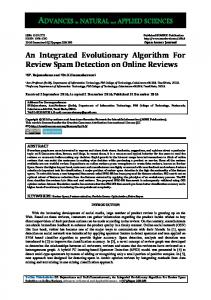
Fig. 1. A three-stage cutting pattern for one bin in normal form.

2

Three-Stage Two-Dimensional Bin Packing

The 2BP problem consists of a set of n rectangular items, each having a height hi and a width wi , i = 1, ..., n. The objective is to pack them into a minimum number of rectangular bins, each having height H and width W . Items may not overlap and we do not consider rotation. A feasible layout for 3-stage 2BP consists of a set of bins, each bin consists of a set of stripes, each stripe consists of a set of stacks, and each stack consists of items having equal width. Every such pattern can be reduced into its so-called normal form by moving each item to its uppermost and leftmost position, so that void space appears only at the bottom of stacks, to the right of the last stack in each stripe and below the last stripe, see Fig. 1. In the sequel we consider only patterns in normal form. In [4] a polynomial-sized ILP model for 2-stage 2BP has been proposed. We extend this model in order to get a polynomial-sized ILP formulation for 3-stage 2BP. The items are sorted so that h1 ≥ h2 ≥ . . . ≥ hn . The order of the items within each stack is not relevant, so they can always be ordered according to their indices. A solution may contain at most n stacks. We label each stack with the index of the highest item it contains, i.e., the smallest item index. Similarly, a solution has at most n stripes, and a stripe’s label is the label of its highest stack. Finally at most n bins are needed and we label each of them with the smallest index of the stripes it contains. The model uses the following 0/1-variables: – – – –

αj,i , j = 1, . . . , n, i = j, . . . , n: rectangle i is contained in stack j; βk,j , k = 1, . . . , n, j = 1, . . . , n: stack j is contained in stripe k; γl,k , l = 1, . . . , n, k = l, . . . , n: stripe k is contained in bin l; δl,i,j , l = 1, . . . , n − 1, i = l + 1, . . . , n, and j = l, . . . , i − 1: item i contributes to the total height of all stripes in bin l; i.e., item i appears in stack j, stack j appears in stripe j, and stripe j appears in bin l.

An EA for Column Generation

3

The 3-stage 2BP problem can now be stated as the following ILP: minimize

n X

γl,l

(1)

αj,i = 1, ∀i = 1, . . . , n

(2)

l=1

subject to

i X

j=1 n X

αj,i ≤ (n − j)αj,j ,

∀j = 1, . . . , n − 1

(3)

i=j+1

αj,i = 0, ∀j = 1, . . . , n − 1 ∀i > j | wi 6= wj ∧ hi + hj > H n X βk,j = αj,j ∀j = 1, . . . , n k=1 n X

hi αj,i
0 if checkNoConflicts(i) induced = recursiveCheck(i) if induced == ∅ pack(bin, i) else tmp = bin packed = pack(tmp, i) if packed forall items j in induced packed = pack(tmp,j) if not packed break if packed bin = tmp Abbreviations: *.h: height of * *.w: width of * *.uh: unused height of * *.uw: unused width of * R: random value ∈ [0, 1)

Function pack(b, i) forall stripes s in b forall stacks a in s if wi == a.w if hi + a.h ≤ s.h pack i into a return true else if a.h + hi − s.h ≤ b.uh ∧ R < 21 pack i into a return true forall stripes r in b if wi ≤ s.uw ∧ hi ≤ s.h create stack containing i, pack it into s return true else if wi ≤ s.uw ∧ hi − s.h ≤ b.uh ∧ R < create stack containing i, pack it into s return true if hi ≤ b.uh create stack containing i pack it into new stripe, pack it into b return true return false

7

1 2

Fig. 2. First fit heuristic respecting the branching constraints.

5

An Evolutionary Algorithm for the Pricing Problem

Since the 2DKP problem is strongly NP-hard, calling the ILP-solver may be very time-consuming. A more sophisticated metaheuristic, performed when FFBC did not find a variable with negative reduced costs and before solving the problem in an exact way, could lead to a faster overall column generation since significantly fewer calls of the ILP-solver may be needed. We decided to apply an Evolutionary Algorithm (EA) operating directly on stripes, stacks, and items. Structure of the EA We use a standard steady-state algorithm with binary tournament selection and duplicate elimination. In each iteration, one new candidate solution is created by always applying recombination, and applying mutation with a certain probability. The new solution replaces the worst solution in the population if it is not identical to an already existing solution. Representation and initialization The chosen representation is direct: Each chromosome represents a bin as a set of stripes, each stripe as a set of stacks, and each stack as a set of item references. Using such a hierarchy of sets makes it easy to ignore the order of items, stacks, and stripes and to avoid symmetries. Initial solutions are created via the FFBC heuristic using randomly generated item orders. These orders are created in a biased way by assigning each item i a random value ri ∈ [0, 1) and sorting the items according to decreasing ri πi .

8

Jakob Puchinger and G¨ unther R. Raidl

Recombination This operator first assigns a random value rs ∈ [0, 1) to each stripe s in the two parent solutions. All these stripes are then sorted according to decreasing rs ps , with ps being the sum of the πi of the items contained in stripe s. The stripes are then considered in this order and packed into the offspring’s bin when they fit into it (i.e., their height is smaller than the remaining unused height of the bin). Identical stripes of both parents appear twice in the ordered list, but they are considered at their first appearance only. When all stripes have been processed, repairing is usually necessary in order to guarantee feasibility. First, the bin is traversed in order to check if items appear twice, the first of these items is deleted. Then, the branching constraints are considered: Items conflicting with others are removed. Afterwards, we try to pack induced items; if this is not possible the corresponding original items are also removed from the bin. Finally, FFBC is applied to the remaining items, possibly improving the solution. Mutation The mutation operator removes a randomly chosen item i from the bin. If the branching constraints induce other items for i, they are also deleted. Finally, FFBC is applied to the remaining items for local improvement.

6

Experimental Results

We performed experiments on the benchmark instances from Berkey and Wang [2] (classes 1 to 6) and Martello and Vigo [7] (classes 7 to 10). We compare CPLEX 8.1 directly applied to the ILP model (1) to (12) and the two variants of the B&P approach with and without the EA for solving the pricing problem. The B&P algorithm was implemented using the opensource framework COIN/Bcp (version 2004/04) [6], the LPs were solved using COIN/Clp. The computational experiments were performed on a Pentium 4 PC with 2.8 GHz. The EA’s population size was 100, the mutation was performed with probability 0.75, and the EA terminated when either 1 000 iterations were performed without an improvement of the best solution or after a total of 100 000 iterations. Each of the experiments had a time limit of 1 000 seconds, which was occasionally exceeded because CPLEX is given the same time limit of 1 000 seconds. Table 1 shows results obtained for the 10 problem classes; in each class there are 50 instances divided into 5 subclasses with n = 20, . . . , 100 items. For each of the considered algorithms (CPLEX, B&P, B&P with EA), average objective values z of finally best integer solutions, numbers of instances solved to provable optimality Opt (out of 10), and average times t in seconds are given. The last rows show totals and averages over all instances. When CPLEX is directly applied to the ILP model, 335 out of 500 instances could be solved to provable optimality. This is not bad, but substantially less than B&P’s 402 instances and in particular the 409 completely solved instances of the EA-enhanced B&P. The differences in the objective values of the finally best integer solutions found by the three algorithms for instances that could not be

An EA for Column Generation

Class

n 20 40 60 80 100 20 40 60 80 100 20 40 60 80 100 20 40 60 80 100 20 40 60 80 100 20 40 60 80 100 20 40 60 80 100 20 40 60 80 100 20 40 60 80 100 20 40 60 80 100

1

2

3

4

5

6

7

8

9

10

Total Average

CPLEX B&P z Opt t [s] z Opt 7.2 10.0 0.0 7.2 10.0 13.6 6.0 404.8 13.6 8.0 20.2 3.0 748.9 20.2 8.0 27.8 0.0 1000.6 27.6 9.0 32.7 0.0 1001.3 32.3 4.0 1.0 10.0 0.0 1.0 10.0 2.0 9.0 100.2 2.0 9.0 2.8 7.0 300.8 2.8 7.0 3.4 7.0 302.4 3.4 7.0 4.1 8.0 206.7 4.1 8.0 5.4 10.0 0.0 5.4 10.0 9.7 8.0 307.2 9.8 9.0 14.2 5.0 704.3 14.2 7.0 20.3 0.0 1000.4 19.5 7.0 23.9 0.0 1000.8 23.2 2.0 1.0 10.0 0.0 1.0 10.0 2.0 9.0 100.1 2.0 9.0 2.6 7.0 353.7 2.7 6.0 3.3 7.0 300.9 3.3 7.0 4.0 7.0 302.0 4.0 7.0 6.6 10.0 0.0 6.6 10.0 12.3 10.0 24.2 12.3 10.0 18.3 10.0 10.3 18.3 10.0 25.0 5.0 530.1 24.8 9.0 29.4 1.0 901.5 28.9 5.0 1.0 10.0 0.0 1.0 10.0 1.9 10.0 14.2 1.9 6.0 2.3 8.0 200.2 2.3 8.0 3.0 10.0 0.4 3.0 10.0 3.6 6.0 400.8 3.6 6.0 5.7 10.0 0.0 5.7 10.0 11.5 6.0 566.3 11.5 10.0 16.2 0.0 1000.2 16.2 9.0 23.5 0.0 1000.4 23.2 10.0 28.0 0.0 1000.7 27.1 10.0 6.1 10.0 0.0 6.1 10.0 11.4 10.0 0.6 11.5 9.0 16.4 10.0 8.6 16.5 9.0 22.6 8.0 288.6 22.7 9.0 28.2 8.0 410.0 28.3 7.0 14.3 10.0 0.0 14.3 10.0 27.8 10.0 0.0 27.8 10.0 43.7 10.0 0.1 43.7 10.0 57.7 10.0 0.2 57.7 10.0 69.5 8.0 200.3 69.5 10.0 4.5 10.0 0.0 4.5 10.0 7.7 9.0 185.8 7.7 9.0 10.7 3.0 822.1 10.7 2.0 14.0 0.0 1000.4 13.9 0.0 16.9 0.0 1000.7 16.9 0.0 741.0 335.0 17702.0 737.5 402.0 14.82 6.70 354.04 14.75 8.04

B&P with EA t [s] z Opt t [s] 0.3 7.2 10.0 6.3 206.1 13.6 8.0 204.0 256.9 20.1 8.0 221.6 182.1 27.6 9.0 183.9 845.6 32.0 6.0 590.4 0.1 1.0 10.0 0.1 113.0 2.0 9.0 118.3 317.9 2.8 7.0 411.2 377.9 3.4 7.0 410.1 344.0 4.1 8.0 220.8 0.2 5.4 10.0 0.3 124.3 9.7 10.0 7.0 386.9 14.1 9.0 184.4 423.9 19.3 8.0 280.2 950.1 22.9 3.0 946.9 0.1 1.0 10.0 0.1 100.7 2.0 9.0 166.6 413.3 2.7 6.0 736.5 402.3 3.3 7.0 303.3 378.2 4.0 7.0 306.9 0.2 6.6 10.0 0.8 23.0 12.3 10.0 3.1 19.0 18.3 10.0 89.0 199.4 24.8 9.0 213.7 621.6 28.9 7.0 536.3 0.1 1.0 10.0 0.1 401.7 1.9 6.0 405.7 202.2 2.3 8.0 201.3 3.1 3.0 10.0 3.1 405.5 3.6 6.0 405.6 0.3 5.7 10.0 0.7 4.9 11.5 10.0 39.7 128.5 16.1 10.0 24.7 60.2 23.3 9.0 157.3 292.1 27.1 10.0 269.6 0.8 6.1 10.0 0.9 133.7 11.4 10.0 120.1 116.0 16.5 9.0 118.6 177.8 22.9 7.0 346.5 506.4 28.4 6.0 508.9 0.1 14.3 10.0 0.2 0.4 27.8 10.0 0.6 1.4 43.7 10.0 1.5 3.6 57.7 10.0 3.8 7.9 69.5 10.0 8.5 0.7 4.5 10.0 0.5 166.1 7.8 8.0 217.4 857.2 10.5 3.0 825.1 1048.8 13.6 0.0 1114.5 1048.5 16.6 0.0 1151.4 12254.9 735.9 409.0 12068.2 245.10 14.72 8.18 241.36

Table 1. Experimental results of the presented algorithms.

9

10

Jakob Puchinger and G¨ unther R. Raidl

solved to optimality are in general relatively small. Nevertheless, B&P’s solution values are in several cases significantly better than those of CPLEX, and the EAenhanced B&P performs best on average. The two variants of B&P with and without the EA exhibit approximately the same total running times. Applying CPLEX directly was significantly slower in most cases. Thus, the application of the EA within the B&P framework is worth the additional effort.

7

Conclusions and Future Work

For 3-stage 2BP, we presented a compact ILP model having only O(n3 ) variables. In practice, however, the proposed column generation approach having a number of potential variables that grows exponentially with n turns out to be more efficient. Using the described EA as an additional strategy for solving the pricing problem pays off in terms of a higher capability of solving instances to provable optimality, but also slightly better average solution values. The combination of B&P and an EA in this form is also highly promising for other combinatorial optimization problems. Research on more sophisticated interaction and a parallel execution of these algorithms will be done next.

References 1. G. Belov and G. Scheithauer. A branch-and-cut-and-price algorithm for onedimensional stock cutting and two-dimensional two-stage cutting. Technical Report MATH-NM-03-2003, Dresden University of Technology, Germany, 2003. 2. J. O. Berkey and P. Y. Wang. Two-dimensional finite bin packing algorithms. Journal of the Operational Research Society, 38:423–429, 1987. 3. P. C. Gilmore and R. E. Gomory. Multistage cutting-stock problems of two and more dimensions. Operations Research, 13:90–120, 1965. 4. A. Lodi, S. Martello, and D. Vigo. Models and bounds for two-dimensional level packing problems. Journal of Combinatorial Optimization. To appear. 5. A. Lodi, S. Martello, and D. Vigo. Recent advances on two-dimensional bin packing problems. Discrete Applied Mathematics, 123:373–390, 2002. 6. R. Lougee-Heimer. The Common Optimization INterface for Operations Research: Promoting open-source software in the operations research community. IBM Journal of Research and Development, 47(1):57–66, 2003. 7. S. Martello and D. Vigo. Exact solutions of the two-dimensional finite bin packing problem. Management Science, 44:388–399, 1998. 8. D. Pisinger and M. Sigurd. Using decomposition techniques and constraint programming for solving the two-dimensional bin packing problem. Technical Report 03/01, University of Copenhagen, Denmark, 2003. 9. J. Puchinger, G. R. Raidl, and G. Koller. Solving a real-world glass cutting problem. In J. Gottlieb and G. R. Raidl, editors, Evolutionary Computation in Combinatorial Optimization – EvoCOP 2004, volume 3004 of LNCS, pages 162–173. Springer, 2004. 10. F. Vanderbeck. A nested decomposition approach to a 3-stage 2-dimensional cutting stock problem. Management Science, 47(2):864–879, 1998. 11. L. A. Wolsey. Integer Programming. Wiley-Interscience, 1998.