A column generation algorithm for a vehicle routing problem with economies of scale and additional constraints Alberto Ceselli, Giovanni Righini∗, Matteo Salani† Dipartimento di Tecnologie dell’Informazione Universit`a degli Studi di Milano Via Bramante 65, 26013 Crema, Italy {ceselli,righini,salani}@dti.unimi.it
Abstract We present an optimization algorithm developed for a provider of software planning tools for distribution logistics companies. The algorithm computes a daily plan for a heterogeneous fleet of vehicles, that can depart from different depots and must visit a set of customers for delivery operations. Besides multiple capacities and time windows associated with depots and customers, the problem also considers incompatibility constraints between goods, depots, vehicles and customers, maximum route length and durations, upper limits on the number of consecutive driving hours and compulsory drivers’ rest periods, the possibility to skip some customers and to use express courier services instead of the given fleet to fulfill some orders, the option of splitting up the orders, and the possibility of “open” routes that do not terminate at depots. Moreover, the cost of each vehicle route is computed through a system of fares, depending on the locations visited by the vehicle, the distance traveled, the vehicle load and the number of stops along the route. We developed a column generation algorithm, where the pricing problem is a particular resource constrained elementary shortest path problem, solved through a bounded bi-directional dynamic programming algorithm. We describe how to encode the cost function and the complicating constraints by an appropriate use of resources and we present computational results on real instances obtained from the software company.
∗ Corresponding † Currently
author:
[email protected] ´ at: Ecole Polytechnique F´ ed´ erale de Lausanne.
1
1
Introduction
The delivery and collection of goods at customers’ locations accounts for a relevant part of the supply chain cost. Optimally planning the distribution of goods is an effective way to obtain substantial savings. In the last decades different optimization techniques have been widely applied to the exact optimization of vehicle routing problems: algorithms based on branch-and-bound, branch-and-cut and branch-and-price have been proposed. A detailed survey on such techniques can be found in the book [27], but this is a still growing research area: recent methods like branch-and-cut-and-price have advanced the state of the art [19] [20]. Exact optimization algorithms based on column generation exploit the DantzigWolfe decomposition of the flow formulation of the original problem into a master problem and a pricing subproblem. The master problem is a partitioning problem with binary variables, while the pricing subproblem is a constrained elementary shortest path problem, which is iteratively solved to produce new promising columns. We address the reader to the recent book [11] on column generation for a review of such methods. Recent contributions have advanced the knowledge on column generation, allowing to get rid of some drawbacks of the method. In particular, dual space stabilization issues have been addressed by Rousseau et al. [26] and Ben Amor et al. [1], dual space cutting planes and constraint aggregation methods have been proposed by Ben Amor et al. [6] and Elhallaoui [17] respectively. Despite all these advances in real-world routing and scheduling applications, several complicating constraints motivated practitioners and researchers to resort to heuristics and meta-heuristics, trading optimality or approximation guarantees for efficiency and flexibility. For instance, Koskosidis [22] addressed the vehicle routing and scheduling problem with soft time window constraints. An exact optimization algorithm for the same problem has been recently presented by Liberatore et al. [23]. Bianchessi and Righini [7] devised a complex and variable neighborhood search algorithm for the vehicle routing with simultaneous pick-up and deliveries, recently attacked also by Dell’Amico et al. [10] with exact optimization algorithms. Within the difficulties issued by real-world problems it is worth to mention split deliveries. In a classical vehicle routing problem the customer can be served by at most one vehicle, while in the VRP with split deliveries (SDVRP) this constraint is relaxed. In an optimal solution of a SDVRP some customers requests can be split up and assigned to several vehicles. Such a relaxation allows to model the case in which the customers demands are greater than the vehicles capacity. The SDVRP has been considered by Dror [16], who also proposed a branch-and-bound heuristic [15]. Some advances regarding the computational complexity, a bound on the cost reduction, and an optimization-based heuristic have been illustrated by Archetti et al. [3] [2] [4]. At the best of our knowledge, the characteristics presented above have never been considered simultaneously by any exact optimization method for vehicle routing problems. Heuristic methods, mainly based on local search, can be found 2
in [28], [21], and [13]. We also refer the reader to the reviews by Gendreau et al. [8] [9]. In this work we consider a real world vehicle routing problem and we illustrate an optimization algorithm based on column generation and dynamic programming. We show that the proposed approach is flexible enough to take into account several complicating constraints and it is able to compute an optimal solution or a near-optimal one with an a posteriori approximation guarantee. In Section 2 we describe the routing problem and its model; in Section 3 we describe how to treat the additional constraints in the dynamic programming algorithm, in Section 4 we discuss some implementation issues and in Section 5 we present computational results.
2
Problem description
The constraints. The distribution network of our problem consists of two types of locations: customer sites and depots. The position of each location is known and defined by a five-levels hierarchical code: nation (e.g. Italy), zone (e.g. North, Center, South), region (e.g. Piedmont, Tuscany), district (e.g. Milan, Florence) and ZIP code. Each location can be defined at any level of detail in the hierarchy: for instance, for some locations only the region is specified, whereas for other locations all data are. The distance between each pair of locations, in terms of both kilometers and traveling time, is known as well. Due to different road types and average traffic conditions, distance in time and in space may not be proportional. For both location types we are given a set of time windows in which loading and unloading operations can take place and the service time needed to perform them. For each customer site we are also given the set of orders that must be delivered and the maximum allowed number of visits to the site for each day. Each order is made of several items; each item consists of goods, organized in pallets; three coefficients describe the characteristics of each item, namely weight, volume and value. Orders can be split but items cannot. Therefore this problem falls in between the single-source vehicle routing problem and the split delivery vehicle routing problem. The problem instances we were given, contained up to 100 orders, 374 items and 137 available vehicles. Therefore the attempt to solve the problem as a single-source VRP with as many vertices as the items would be impractical. The daily duty of each vehicle of the fleet can be composed of many routes, each starting at the same depot. The vehicles have several characteristics: a maximum weight, volume, value and number of pallets that the vehicle can load; a maximum daily duty length (in terms of both time and distance); a maximum length for each route (in terms of both time and distance); a limit on the number of allowed stops along the route. By stop we mean a visit to a customer to execute a delivery operation.
3
Constraints are imposed on the time needed for loading items at the depot and unloading them at the customers; the time is computed as a weighted sum of the number of pallets, weight, volume and value of the goods. Therefore the departure time of a vehicle from the depot depends on the amount of carried goods. Each item may not be available in all the depots. Moreover, each vehicle can be incompatible with a given set of items, representing for instance hazardous or fragile goods, and with some locations. Because many vehicles share the same characteristics, we found useful to group identical vehicles into vehicle sets of a given type. The computation of route schedules is particularly involved: each vehicle spends time in traveling from a location to another, by waiting to access the locations and by loading and unloading goods. There are strict rules for the rest periods: each driver has to rest for 45 minutes every 270 minutes driving. This rest period can be split into shorter breaks: the waiting time and loading/unloading time count as a break only if they amount to at least 15 minutes without interruption. Further incompatibilities exist between items and between items and locations. It is common practice that some goods are not transported with some others on the same vehicle, for instance food and detergents, although the vehicle itself is allowed to transport both types of goods. In a feasible plan each order must be delivered, but the planner has the option of paying an express courier for distributing some of the items. This option has to be used as an exception, because the costs of the courier are higher than those of the available vehicles. However in some cases it may happen that small amounts of goods should be delivered to customers far away from the depot and isolated from other customers, so that no economies of scale are possible. In these exceptional cases it may be cheaper to send the items via express courier. A complete plan is computed with daily frequency. The cost function. A cost is associated with each vehicle route, and it is computed through a non trivial system of fares. There are six different types of fares depending on the following six characteristics of the route: 1. the total number of pallets carried, 2. the total weight, 3. the total volume, 4. the total value, 5. the overall traveled distance, 6. the number of stops. In order to model economies of scale, each fare is defined by ranges. Each range is described by a lower limit, an upper limit, a fixed cost and a unitary cost; 4
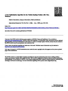
for each route and for each of the former five characteristics, a range is active whenever the value of the characteristic for that route falls between the lower and the upper limit. The fixed cost and the unit cost of the active range define the fare for that route for for that characteristic. The fares on the number of stops are treated in a slightly different way: a given number of stops are free and a given unit cost is added only for each exceeding stop. Finally, each fare is only applied to a given subset of locations: a whole nation, a zone, a region, a district or a single ZIP area. Whenever two (or more) fares related to the same characteristic match the same location, the less specific fares are disregarded. This complicated cost structure implies that each location can have a different set of fares, and a different cost for a route can be computed by considering the fare of each visited location. For each location along the route the six fares related to the six characteristics listed above are added up, yielding the cost of the route for that location. The overall cost of the route is the maximum among the costs corresponding to the locations along the route. In Figure 1 we report a simplified example of such a hierarchical fare system. Italy is split in three zones: North, Center and South. Piedmont and Lombardy are two regions in the North; Turin (TO) and Cremona (CR) districts belong to Piedmont and Lombardy respectively. The ZIP code 26013 correspond to the city of Crema in Cremona district. Seven fares are represented between brackets; each of them has a corresponding characteristic (stops, weight or value), a range (indicated between square brackets), fixed (F) and unit (U) costs in Euro. We consider a vehicle carrying an overall weight of 8 units, whose value is 5000. It performs 2 stops along its route: the first one in Crema and the second one in Rivoli, a town of the Turin district. The national fare on the number of stops does not apply, since its range starts from 3. The vehicle visits Crema, its carried weight (that is 8) falls in the range of the ZIP fare ([0..10]), and the less specific fare for Lombardy is disregarded. At the same time its carried value (that is 5000) falls in the range of the regional fare ([0..20000]); the value fare related to Milan is disregarded, since the vehicle does not stop in Milan district. Considering the first visited location, the route would cost 100 + 30 · 8 EUR for the weight plus 5000 · 0.2 EUR for the value, that is 1340 EUR overall. The vehicle also stops in Rivoli: the Turin weight fare does not apply, since it starts from 25; considering the second visited location the route cost would be 150 + 10 · 8 EUR due to the region weight fare, that is 230 EUR. The final cost of the route is the maximum of these two values, that is 1340 EUR (the cost for the first location). To summarize, the actual cost related to a location j can be obtained by visiting the tree represented in Figure 1 from the leaf representing location j up to the root, and stopping as soon as a matching range (if any) is found. This is like defining a stepwise linear cost function ϕj for each location j, which maps the six characteristic values described above to the cost of the route; the final cost function is obtained as the maximum of the ϕj functions related to the visited locations.
5
Figure 1: Example of the fare system
3
A column generation algorithm
Let P be the set of vehicle types, V be the set of locations, D be the set of depots; S for each location v ∈ V let Qv be the corresponding set of items and let Q = v∈V Qv be the whole set of items to be delivered. We model our problem as a set covering problem (SCP), in which each column encodes a feasible vehicle duty, defined as a sequence of routes for that vehicle: X X minimize ck z k (1) p∈P k∈Ωp
s.t.
X X
xkq z k ≥ 1
∀q ∈ Q
(2)
∀p ∈ P
(3)
∀v ∈ V
(4)
∀p ∈ P, ∀k ∈ Ωp
(5)
p∈P k∈Ωp
X
z k ≤ np
k∈Ωp
X X p∈P
skv z k ≤ mv
k∈Ωp
z k ∈ {0, 1}
In this model Ωp is the set of feasible duties that can be assigned to a vehicle of type p in one day. Each coefficient xkq is 1 if item q is delivered along a route in duty k, 0 otherwise: covering constraints (2) impose that each item is delivered. Each term np represents the maximum number of vehicles of type p available per day: constraints (3) replace convexity constraints, by limiting the number of duties assigned to vehicles of the same type. Each term mv represents the maximum number of visits allowed to location v during the same day, and each term skv represents the number of visits to location v performed during duty k: constraints (4) ensure that the number of routes entering each location does not exceed the maximum allowed number of daily visits. The remaining constraints are encoded in the construction of the sets Ωp of feasible duties. For each duty k ∈ Ωp the variable z k takes value 1 if duty k is selected, 0 6
otherwise. The cost ck of each duty k is computed through the system of fares described in the previous section, and the objective (1) is to select a feasible subset of duties in order to minimize the overall operating costs. The pricing problem. The set covering model may contain a number of variables which grows combinatorially with the size of the instance. In order to compute a valid lower bound, we have recourse to column generation. For a detailed treatment of column generation applied to vehicle routing problems we refer the reader to the recent book edited by Desaulniers et al. [11]. In particular we relax integrality conditions and we consider a restricted set covering problem (RSCP). Initially it includes only |Q| columns, one for each item q, with a coefficient 1 in the corresponding covering constraint, and 0 elsewhere. The cost of these columns is known in advance and it corresponds to the fare of the express courier which is known. The presence of these columns ensure that a feasible solution always exists for the RSCP independently of the columns generated dynamically. At each column generation iteration the linear relaxation of the RSCP is solved and we search for new columns with negative reduced cost. The reduced cost of each column k ∈ Ωp can be computed as: X X c¯k = ck − πq xkq − δp − γv skv q∈Q
v∈V
where πq is the non-negative dual variable associated to the q-th constraint of the set (2), δp is the non-positive dual variable associated to the p-th constraint of the set (3) and γv is the non-positive dual variable associated to the v-th constraint of the set (4). Hence, instead of explicitly computing the reduced cost of all the variables in the problem, we solve several pricing problems, one for each p ∈ P and for each d ∈ D, in order to identify one or more negative reduced cost columns; this corresponds to search for feasible duties with negative reduced cost for each vehicle type and for each starting depot. If columns with negative reduced cost are found, they are inserted into the RSCP and the process is iterated; otherwise, the optimal fractional solution of the linear relaxation of the RSCP is also an optimal solution of the linear relaxation of the SCP.
3.1
A pricing algorithm
The pricing problem is a special case of the resource constrained elementary shortest path problem (RCESPP) formulated on a graph having one vertex for each item, non-negative costs on the arcs, non-positive prizes on the vertices (given by the πq dual variables) and non-negative penalties for entering each location (given by the γv dual variables). We also set γσ = γτ = 0. Both orders and locations correspond to subsets of items, and therefore to subsets of vertices of the graph. In Section 4 we describe how to exploit this relation to design smart aggregation schemes. 7
The RCESPP is known to be strongly NP-hard [14]. The most commonly used technique to solve the RCESPP to optimality is dynamic programming, relying upon the seminal work by Desrochers and Soumis [12], in which a relaxation of the pricing algorithm is solved, where cycles are allowed. Recently Righini and Salani [24] proposed dynamic programming algorithms in which the pricing problem is solved exactly, without allowing for cycles. In this work we adapted the bounded bi-directional dynamic programming (BBDP) algorithm proposed by Righini and Salani, to solve our pricing problem to optimality, encoding all the constraints through suitable resources. The BBDP algorithm generates separately forward and backward partial paths from and to the depot as labels of a dynamic programming algorithm. The extension of forward and backward paths is defined in such a way that one half of the vehicle routes in one duty is performed forward and one half backward; furthermore, if the number of routes is odd, half of the stops in the central route are visited forward and half backward. The BBDP algorithm keeps a list of non-dominated labels, grouped for each order, and iteratively extends labels retaining only the Pareto-optimal ones according to a dominance criterion. Each time a certain number of labels is created, the algorithm builds complete paths by joining compatible forward and backward partial paths. Hereafter we describe how we have encoded the constraints by means of resources, while in the next subsections we detail how the extension and joining steps are performed. When considering vehicle type p and depot d we discard items which are either unavailable at depot d or incompatible with vehicle type p. We represent each item as a vertex i ∈ I; two more vertices σ and τ represent the depot where the vehicle duty starts and ends. We assign to each vertex i a set of states, representing routes from the starting vertex σ to vertex i. Each state includes a resource consumption vector R, whose components represent the quantity of each resource used along the corresponding route. In our case, this resource vector has the following components: • traveled distance (l) • number of stops (b) • number of loaded pallets (p) • weight of loaded items (w) • volume of loaded items (v) • value of loaded items (c) Moreover, in each state we keep track of the time spent in driving (tl ) and resting (tb ) along the route. Owing to the contribution of the πq dual variables to the route cost, our graph may contain negative cost cycles. In order to generate elementary paths only, as proposed by Beasley and Christofides [5] we attach to labels a set V ,
8
representing the visited locations, a set S of delivered items and a set Σ of items which are incompatible with the delivered ones. Each state has an associated cost C, depending on traversed arcs and visited locations, and a prize ζ depending on the πq and γv dual variables associated with the visited locations; an optimal solution corresponds to the state associated with vertex τ with minimum value of C − ζ. Hence in our algorithm each state is represented by a label of the form (S, Σ, V, R, tl , tb , C, ζ, i); the initial state representing an empty vehicle at the depot is encoded with a label (∅, ∅, ∅, [0 . . . 0], 0.0, 0.0, 0.0, 0.0, σ). Extension. Our algorithm repeatedly extends each label to generate new labels. In particular, the extension of a label (S, Σ, V, R, tl , tb , C, ζ, i) corresponds to appending an additional arc (i, j) to a path from σ to i, obtaining a path from σ to j. The extended label has the form (S 0 , Σ0 , V 0 , R0 , t0l , t0b , C 0 , ζ 0 , j). We remark that vertices i and j correspond to specific items, and therefore to specific amounts of goods delivered. Hence, we indicate extensions from a vertex i to a vertex j corresponding to items in the same location as internal extensions. On the opposite, we indicate extensions from a vertex i to a vertex j corresponding to items in different locations as external extensions. Therefore, each path is built by many extension blocks, each composed by an external extension and a sequence of internal extensions. The sequence of internal extensions in each block defines a set Θ ⊆ Q of delivered items, and this set is included in the encoding of the state. In order to avoid exploring many symmetric solutions, we define a partial order, in which each item corresponding to a vertex i in location l preceeds items corresponding to each vertex j > i in the same location, and we do not allow internal extensions from any vertex j to any vertex i with i < j. The actual consumption of resources can be computed only when the whole extension block is performed. In fact, as described below, its value depends both on the location of the customer identified during the external extension and on the set Θ of items delivered during the sequence of internal extensions. Let (i, j) be the arc appended during the external extension of the block. With an abuse of notation, we indicate as lij (resp. tij ) both the distance (resp. travelling time) between locations i and j and the distance between the locations corresponding to vertices i and j. The traveled distance is updated as R0 (l) = R(l)+lij , and the number of stops is increased by one: R0 (b) = R(b)+1. Then we represent the consumption implied by each item q ∈ Θ as a vector ρq with the following four components: • number of unloaded pallets (p) • weight of unloaded items (w) • volume of unloaded items (v) • value of unloaded items (c). 9
P We update the route resource consumption as follows: R0 (α) = R(α)+ q∈Θ ρq (α), for each of the four characteristics α ∈ {p, w, v, c}. The computation of the rest time and driving time is more involved: first, we have to take into account work rules, that impose to take one break 45 minutes long after each uninterrupted driving period of 270 minutes. Drivers are allowed to take breaks at any point along the route. Hence, while moving from i to j, the number of breaks to be made is given by b = max{b(tl + tij )/270c − btb /45c, 0} and the arrival time at vertex j is tl + tb + tij + b · 45. Because each location j has a time window starting at aj , in case of early arrival the vehicle has to wait until the starting time of the time window and then the arrival time is set to aj . Finally, let u(Θ) be the time spent for unloading operations: the unloading time per pallet and per unit of weight, volume and value is given; hence u(Θ) can be directly computed from input data. According to the work rules, if δ + u(Θ) ≥ 15 the waiting and unloading time counts as rest time, otherwise it counts as driving time. Therefore the time resources are updated as follows: if δ + u(Θ) ≥ 15, then t0l = tl + tij and t0b = t0b + b · 45 + δ + u(Θ); otherwise t0l = t0l + tij + δ + u(Θ) and t0b = t0b + b · 45. We remark that, according to these rules, a driver may accumulate resting time by anticipating a break, but he can not delay a break. However anticipating breaks when it is not needed is always a suboptimal choice. Finally, it is never convenient to serve a same location in more than one round, since coming back only implies additional resource consumption. Let v be the location corresponding to vertex j: we set V 0 = V ∪ {v} and S 0 = S ∪ Θ; moreover we include in Σ0 the items in Σ∪Qv and any item which is incompatible with an itemP in Θ. We also set Θ = ∅. The prize ζ 0 of the new label is computed 0 as ζ = ζ + q∈Θ πq + (γi + γj )/2. Instead, the cost C 0 is computed from the set of visited locations V 0 through the system of fares described in Section 2. Feasibility. Each vehicle has a limited capacity, which is separately given in terms of maximum number of loadable pallets, weight, volume and value. Each subset of items Θ yielding a state in which these limits are violated is not considered during the internal extensions. Then, if the closing time bj of a location is exceeded, that is t0l + t0b > bj , the corresponding label is discarded. Moreover, a maximum travel distance, time duration and number of stops are imposed to each route: whenever one or more components of the R0 vector exceed these limits, the corresponding label is not created. In order to avoid cycles, we do not consider any location j ∈ S during extension. Finally, since each vehicle has to come back to the depot, if R0 (l)+ljτ exceeds the maximum travel distance or t0l + t0b + tjτ exceeds the maximum travel time, we discard the new label. If a given vehicle is allowed to perform open routes, this is taken into account by setting ljτ = 0 for all vertices j for that vehicle. Furthermore, exploiting an idea of Feillet et al. [18] we include in Σ0 the set of items placed in any location e such that R0 (l) + lje + leτ exceeds the maximum travel distance or t0l + t0b + tje + teτ exceeds the maximum travel time
10
(Σ0 = Σ0
S
Qe ).
Dominance. The effectiveness of the dynamic programming algorithm heavily depends on the number of states generated. Hence it is essential to fathom feasible states which cannot lead to the optimal path. To this purpose suitable dominance tests are always performed when states are extended, so that the algorithm records only non-dominated states. After each internal extension the we perform a simplified dominance test: let Θ0 and Θ00 be two item sets associated with vertex i during internal extensions 0 of the same label. A state a state in which P in whichPΘ is deliveredPdominates P 00 Θ is delivered only if q∈Θ0 ρq ≤ q∈Θ00 ρq and q∈Θ0 πq ≥ q∈Θ00 πq . Instead, after each extension block, the actual resource consumption is known, and the set Θ is empty; therefore we perform the following complete dominance test. Let ς 0 = (S 0 , Σ0 , V 0 , R0 , t0d , t0b , C 0 , ζ 0 , i) and ς 00 = (S 00 , Σ00 , V 00 , R00 , t00d , t00b , C 00 , ζ 00 , i) be the labels of two states associated with vertex i. State ς 0 dominates ς 00 only if V 0 ⊆ V 00 S 0 ∪ Σ0 ⊆ S 00 ∪ Σ00 R0 ≤ R00
(6) (7) (8)
t0d ≤ t00d
(9)
0d
0b
00d
00b
t +t ≤t +t C 0 + ζ 0 ≤ C 00 + ζ 00
(10) (11)
Furthermore, at least one among the inequalities and the inclusions has to be strict. In particular, if conditions (9) and (10) are satisfied, this means that state ς 0 corresponds to a route in which the driver has spent less time in driving and it has taken less time to perform the same route as in state ς 00 ; moreover, one can easily check that no more breaks have to be made after ς 0 than after ς 00 . In fact, suppose t0b ≤ t00b (and δ = t00b − t0b ), then R0 (t) + δ = t0l + t0b + (t00b − t0b ) = t0l + t00b ≤ t00l + t00b = R00 (t); in other words, the driver in state ς 0 can rest as much as the driver in state ς 00 , and still it takes less time to perform the route. Moreover, this condition is less strict than imposing t0b ≥ t00b , and therefore may yield tighter dominance. We remark that although the computation of the cost function is very involved, when the above conditions are satisfied inequality (11) still guarantees that no better state can be obtained by extending ς 00 instead of ς 0 . In fact, as described in Section 2, the set of fares related to a location j defines a stepwise linear cost function ϕj (R); therefore, the cost of the first state is computed as f 0 (R) = maxj∈V 0 {φj (R)} and the cost of the second state is computed as f 00 (R) = maxj∈V 00 {φj (R)}. Since V 0 ⊆ V 00 , f 0 (R) ≤ f 00 (R) for each R.
11
Bidirectional Dynamic Programming. The combination of bi-directional search with resource-based bounding allows to solve larger instances (or the same instances in less time) than mono-directional dynamic programming; detailed experimental results are reported in [25]. Instead of starting with just one initial state, we create two initial states (∅, ∅, ∅, [0 . . . 0], 0.0, 0.0, 0.0, σ) and (∅, ∅, ∅, [0 . . . 0], 0.0, 0.0, 0.0, τ ), marked ‘forward’ and ‘backward’ respectively. Each forward state is extended as described before, generating further forward states. The extension of backward states follows symmetrical rules; it differs only in the computation of the rest time and the driving time: first, we swap the aj and bj values in the computation of the waiting time and in the feasibility test. Moreover, let ς 0 = (S 0 , Σ0 , V 0 , R0 , t0d , t0b , C 0 , ζ 0 , i) and ς 00 = (S 00 , Σ00 , V 00 , R00 , t00d , t00b , C 00 , ζ 00 , i) be the labels of two backward states associated with vertex i, such that t0d ≤ t00d and t0d + t0b ≤ t00d + t00b . According to the dominance criteria, ς 0 may dominate ς 00 . However, extending both states backward it may happen that the driving time between two breaks in the extended ς 0 state exceeds the limit of 270 minutes, while it does not when ς 00 is extended. This may happen even if t0b > t00b . Hence, in the dominance test between backward states, we tighten condition (10) as follows: t0d + t0b + 45 ≤ t00d + t00b . When no more forward or backward feasible non-dominated states can be generated, complete paths are obtained by joining forward and backward labels. A forward label ς 0 = (S 0 , Σ0 , V 0 , R0 , t0l , t0b , C 0 , ζ 0 , i) and a backward label ς 00 = (S 00 , Σ00 , V 00 , R00 , t00l , t00b , C 00 , ζ 00 , j) can be joined to yield a complete route only if V 0 ∩ V 00 = ∅ and (S 0 ∪ Σ0 ) ∩ (S 00 ∪ Σ00 ) = ∅, that is no location is visited twice, no item is delivered twice and no pairs of incompatible items are transported together; moreover, the resource consumption R on the whole route is computed as R(α) = R0 (α)+R00 (α) for each α ∈ {b, p, w, v, c} and R(l) = R0 (l)+R00 (l)+lij . Setting b = max{b(t0l + tij )/270c − bt0b /45c, 0}, the overall time spent in driving is tl = t0l + tij + t00l and the overall resting time is tb = t0b + 45 · b + t00b . In order the join to be feasible each component of R, and the driving and overall time must not exceed the resource consumption upper bound. ¯ Let R(b) be the maximum number of stops allowed during a route. We ¯ discard forward and backward states in which respectively more than dR(b)/2e ¯ and more than bR(b)/2c stops are performed, since every feasible route can be ¯ obtained by combining the remaining states. When R(b) is odd, we allow more stops in forward states, since backward dominance criteria are weaker (they are given by tighter sufficient conditions). The prize of the route is ζ 0 + ζ 00 and the cost of the route is computed considering the vector R and the set of locations V 0 ∪ V 00 . Handling multiple routes per duty. In the general setting, each vehicle may perform many routes in the same duty, provided it comes back to the depot for loading operations. We take into account multiple routes by introducing the following resource in the resource vector of each label: 12
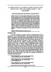
• overall traveled distance (L) • overall elapsed time (T ) • number of completed routes (N ). which are reset to 0 in the initial states. Coming back to the depot in a forward state from vertex i is represented by an extension to the vertex τ . In this case, the new resources are updated as • R(L) = R(L) + R(l) • R(T ) = R(T ) + td + tb + 45 · max{b(td + tiτ )/270c − btb /45c, 0} • R(N ) = R(N ) + 1 • V =∅ • Σ=∅ and all the other components are set to 0. Coming back to the depot in a backward state is represented by a similar extension to vertex σ, and R(T ) = R(T ) + td + tb + 45 · max{b(td + tτ i )/270c − btb /45c, 0}. ¯ , we allow at If the number of allowed routes in each duty is limited to N ¯ /2e routes in both forward and backward states; when N ¯ is odd, we most dN ¯ ¯ limit the number of stops in the last route to dR(b)/2e and bR(b)/2c in forward and backward states respectively. Implementation issues. Since the cost computation is repeated for each label, in a preprocessing step we create a list of non-dominated fares for each location, where a fare is non-dominated if no more specific fare for the same characteristic covers its entire range. Then, the cost computation can be implemented by scanning the list of each visited location, and summing up the contributions of all the fares whose range matches. In Figure 2 we report the list of fares corresponding to the example in Section 2. The list of labels at each vertex is kept lexicographically ordered. Given two distinct labels ς 0 and ς 00 , we say ς 0 < ς 00 if ς 0 preceeds ς 00 according to this lexicographical order, ς 0 > ς 00 otherwise. In particular, the following resources are considered, from the most significant to the least significant one: N , b, tl +tb , tl , R(l), R(p), R(w), R(v), R(c). When a new label ς 0 is created at vertex i, we scan the corresponding list: for any label ς 00 < ς 0 we check if ς 00 dominates ς 0 ; as soon as a label ς 00 is found, which does not preceed ς 0 in the lexicographycal order, ς 0 is inserted into the list before ς 00 ; finally, for any label ς 00 > ς 0 we check if ς 0 dominates ς 00 . Instead of combining forward and backward paths only when no more labels are created, we try to build complete paths each time the number of forward and backward labels reaches a multiple of a constant value (which we fixed to 5000, according to preliminar experiments). This allows us to identify negative reduced cost columns before the pricing algorithm is completed. In principle, 13
Figure 2: List of fares for different locations each pair of forward and backward labels have to be checked during these combining rounds. However, as described in [25] we use the reduced cost of the best column found so far as a bound, to avoid checking each pair of labels. Instead of exactly solving the pricing problem at each column generation iteration, we try to obtain approximate solutions by relaxing the domination criteria. In particular, we replace conditions (6) and (7) as follows. We define two measures of quality of a partial path: η1 = C−ζ |V | , that is the reduced cost C per visited location, and η2 = R(p) , that is the cost per loaded pallet. The first measure tries to identify partial paths that may yield negative reduced cost columns, while the second one reflects a characteristic of routes which are considered appealing in the currently implemented plan. When two labels ς 0 and ς 00 are considered, ς 0 can dominate ς 00 only if α · η10 + (1 − α) · η20 ≤ α · η100 + (1 − α) · η200
(12)
with α ∈ [0..1]. Setting α = 0.1 produced best results in our case. Finally, we do not solve the pricing problem for each vehicle type p and each depot d at each column generation iteration: if a particular call to the pricing algorithm does not produce columns with negative reduced cost are found, the corresponding pair (p,d) is marked tabu, and no pricing algorithm is called for (p,d) for a certain number of iterations. According to preliminary computational results, we set such value to 5.
4
The optimization algorithm
Our column generation algorithm works in three distinct phases: the first phase is a heuristic column generation with no order splitting, the second phase allows splitting some of the orders and the third phase allows complete splitting. Since there are rather tight computational time limits to compute a plan, the user 14
is allowed to stop the planner at any moment, retaining the best incumbent solution. First phase. The first phase aims at producing feasible solutions quickly. For this purpose we only generate columns corresponding to duties in which no order is split. This is done by solving the pricing problem on a graph in which vertices corresponding to items in the same order are contracted to a single vertex. Let Oi be the set of items corresponding to order i: each macro-item i P created in this way has a delivery prize π and a resource consumption q q∈Oi P ρ . Incompatibilities between each item and particular locations, vehicles q q∈Oi or other items are extended to the whole order. Since all the items of the same order are placed in the same location, no further adjustment is required. When this column generation phase is over, we run a primal heuristic to compute an integer heuristic solution for the whole problem. This heuristic consists in solving to optimality the RSCP with binary-valued variables. To this extent we used a general purpose solver. As discussed in Section 5, on the real instances provided by the software company this first phase typically took a few seconds and the solutions found were a few percentage points far from optimality. Furthermore, they have the important property of being simple to implement for the drivers, because they do not imply order splitting. Second phase. In the second phase we allow orders to be split into single items, but to reduce the computational effort we merge small items at the same location in larger ones. This is done as before by solving the pricing problem on a contracted graph. The merging threshold is a user-defined parameter: from our experiments we found that setting the threshold equal to 20% of the capacity of the smallest vehicle of the fleet was a good and robust choice. Since each column generated in the first phase still represents a feasible duty, we keep all of them for a warm start of the second phase. When also the second column generation phase is over, we run the general purpose solver on the binary RSCP again, generating a new feasible solution. Third phase Finally, we generate columns allowing for full order splitting, using all the columns generated during the first two phases as a warm start and we run the primal heuristic once again at the end of the optimization. Primal heuristics. Given a fractional RSCP solution, we run a simple greedy heuristic in order to identify good integer solutions. First, we fix the value of all the z k variables to 0 and set ϑ = Q; then we iteratively compute a pseudocost c˜k for each variable k in the RSCP, select the column k ∗ = argmin{˜ ck }, fix k∗ k k variable z to 1 and set ϑ = ϑ \ Q , where Q is the set of uncovered items which are covered by column k; we stop as soon as a feasible integer solution is ∗ found, or c˜k is +∞. Each feasible integer solution, which is found to improve the primal bound, is kept as the new incumbent solution. We experimented three policies for defining the pseudo-costs c˜k : •
ck |ϑ∩Qk |
if |ϑ ∩ Qk | > 0
+∞
otherwise
( k
c˜ =
15
•
( −¯ zk c˜ = +∞ k
if |ϑ ∩ Qk | > 0 otherwise
where z˜k is the value of variable z k in the last fractional RSCP solution. • k
c˜ =
( (1 − z˜k ) ·
ck |ϑ∩Qk |
+∞
if |ϑ ∩ Qk | > 0 otherwise
This heuristic is run once for each definition policy of the c˜k pseudo-costs, after each column generation iteration in all the three phases.
5
Computational results
The optimization module has been developed in ANSI C. We used the opensource general purpose solver GLPK for solving both the LP subproblems and the binary RSCP instances arising in the primal heuristics. The following tests were run on a Linux workstation equipped with a Pentium IV 1.6 GHz CPU and a 512 MB RAM. Our optimization module was compiled using gcc 4.1 with full optimizations. We imposed a time limit of 4 hours to each test. In our experimental campaign we rebuilt the application scenario as follows. We considered two datasets (A and B), provided by the software company, each composed by 35 instances. These involve the delivery of a number of order ranging from 10 to 100, with up to 461 different items, and are extracted on a geographical basis, by considering deliveries on the same district, province, region and so on. Instances in dataset A refer to the italian city of Bologna and the surrounding region Emilia–Romagna, while instances in dataset B refer to Milan and Lombardy. They represent typical daily tasks for the planner. In tables 1 and ?? we report our computational results. Each table reports on the geographical data in the columns labeled with D and L, which represent the number of districts and the number of locations, respectively. For each optimization phase we report the size of the instance in terms of number of orders, number of packed items and number of items, within columns labeled with # Orders, # Item blocks and # Items. Columns labeled with UB report on the value of the best known solution obtained in each optimization phase while columns labeled with Time and Cols report on the computational time and on the number of columns generated. In columns labeled with Quality, we reported a measure of the quality of the solution against a valid lower bound for the relative optimization phase, which does not represent a valid lower bound for the original instance, lower values corresponds to high quality. In column LB(3) we report the value of a valid lower bound for the whole instance, when found within the computational time limit. This technique yields primal solutions as well as a valid lower bound on the optimal value. It is evident from the first optimization phase that even instances
16
with 50 packed orders are hard to solve. The involved fare system described in section 2 makes the solution of the pricing subproblem time consuming. We can affirm that the two proposed optimization based heuristics obtained a good valid solution in a reasonable computational time. For instance I20, for example, the best known value has been computed by the first phase in 6.13 seconds, which is just 0.08% from the known valid lower bound. The same value has been computed by the optimization algorithm in almost 3 hours. For some other instances (i.e. instances I21 and I23) the algorithm failed to prove a strict lower bound and, by consequence, the relative quality is low. The additional complexity of splitted items can be showed comparing computational times of the first and the second optimization phases. Some instances have been solved in some seconds for the first phase while they required almost 3 hours in the second phase.
6
Conclusions
We presented an optimization algorithm based on column generation developed for a provider of software planning tools for distribution logistics companies. The algorithm computes a daily plan for a real world vehicle routing problem where an heterogeneous fleet of vehicles, that can depart from different depots, must visit a set of customers for delivery operations. Several operational difficulties that arise in real world application have been addressed such as: multiple capacities, time windows associated with depots and customers, incompatibility constraints between goods, depots, vehicles and customers, maximum route length and durations, upper limits on the number of consecutive driving hours and compulsory drivers’ rest periods, the possibility to skip some customers and to use express courier services instead of the given fleet to fulfill some orders, the option of splitting up the orders, and the possibility of “open” routes that do not terminate at depots. We encoded those operational constraints and the cost function by an appropriate use of resources of a constrained shortest path problem and we solved with a bi-directional dynamic programming algorithm. we presented some computational results on real instances obtained from the software company. Although many features and constraints of the problem were specified during the development of the algorithm, the method proved robust enough to cope with all the additional requirements introduced. Our industrial partners are currently embedding an ANSI C implementation of the algorithm in a decision support system for an Italian transportation company, which operates at a national level.
References [1] H. Ben Amor. Stabilization de l’Algorithme de G´en´eration de Colonnes. ´ PhD thesis, Ecole Polytechnique de Montr´eal, 2002.
17
18
inst. I1 I2 I3 I4 I5 I6 I7 I8 I9 I10 I11 I12 I13 I14 I15 I16 I17 I18 I19 I20 I21 I22 I23
D 1 1 1 1 1 20 1 1 1 1 1 20 20 1 20 1 20 20 20 20 20 20 1
L 1 1 2 4 3 8 6 3 4 1 8 13 16 8 20 7 30 34 29 3 33 47 7
First Phase # Orders 1 2 2 8 10 10 10 10 11 11 18 20 30 30 40 50 50 60 70 80 90 100 100 UB(1) 270.00 110.00 160.00 306.00 460.00 730.00 280.00 621.00 480.00 813.00 1716.00 79222.00 2213.00 1008.00 11130.00 869.00 369453.20 221739.07 9946.01 113635.01 143750.01 655753.01 314249.00
Time(s) 0.05 0.03 0.03 1.85 1.24 0.26 0.30 1.41 205.64 8.71 0.27 6.13 7.42 8995.78 1076.43 13001.00 90.11 1106.81 11126.20 1.26 1338.74 11377.49 11470.35
cols 10 13 14 1644 642 57 264 492 4904 785 117 1821 743 8919 3533 15346 397 4664 8248 24918 9438 6801 9950
Second Phase # Item blocks 1 1 3 8 6 15 21 35 23 26 29 52 37 70 81 33 92 132 95 133 160 174 323 UB(2) 270.00 110.00 160.00 306.00 460.00 730.00 280.00 621.00 480.00 813.00 1716.00 79222.00 2189.00 1008.00 11130.00 338.00 369446.00 221739.07 9946.01 113635.01 110941.97 655753.01 314249.00
Quality 0.0% 0.0% 0.0% 0.0% 0.0% 0.0% 2.4% 1.2% 8.9% 2.3% 23.1% 0.2% 0.0% 6.9% 7.3% 7.0% 0.0% 0.0% 0.1% 7.1% 27.5% 0.1% 86.0%
Table 1: Computational results on dataset A
Quality 0.0% 0.0% 0.0% 0.0% 0.0% 0.0% 0.0% 2.8% 17.2% 11.2% 20.7% 0.0% 0.0% 12.1% 1.9% 13.0% 0.0% 0.1% 1.8% 0.7% 78.6% 0.1% 3.2%
Time(s) 0.04 0.03 0.04 2.37 0.56 0.25 35.29 12809.03 11647.56 11492.90 23.64 11994.87 6.57 11625.42 11241.28 11723.95 11470.39 13001.01 13001.01 2628.93 5273.33 11047.78 202.88 15 39 2566 932 92 2606 6088 7883 1721 398 7251 1451 22816 12661 11358 576 20932 15598 24650 33002 21984 1417
cols
Third Phase # Items 2 5 3 29 26 29 25 54 33 31 56 90 92 89 129 158 164 255 214 343 347 374 461
UB(3) 270.00 110.00 160.00 306.00 460.00 730.00 280.00 621.00 480.00 813.00 1716.00 79222.00 2189.00 1008.00 11130.00 338.00 369446.00 221739.07 9946.01 113635.01 110941.97 655753.01 314249.00
LB(3) 270.00 110.00 160.00 460.00 730.00 272.46 1229.05 79005.10 -
Time(s) 0.04 0.05 0.04 9038.57 2832.81 1.49 7343.35 9042.03 13001.00 11907.72 12093.10 11592.60 8997.28 13001.00 11120.00 939.76 13001.00 9255.82 9190.57 -
cols 19 80 49 12366 10441 345 5248 15054 6525 1795 3688 9529 6797 19668 25632 6558 399 23778 20727 -
[2] and M.W.P. Savelsbergh and M.G. Speranza. Worst-case analysis for split delivery vehicle routing problems. Transportation Science, 40(2):226–234, 2006. [3] and R. Mansini and M.G. Speranza. Complexity and reducibility of the skip delivery problem. Transportation Science, 39(2):182–187, 2005. [4] C. Archetti, M.W.P. Savelsbergh, and M.G. Speranza. An optimizationbased heuristic for the split delivery vehicle routing problem. Technical report, Department of Quantitative Methods, University of Brescia, 2006. [5] J.E. Beasley and N. Christofides. An algorithm for the resource constrained shortest path problem. Networks, 19:379–394, 1989. [6] Hatem Ben Amor, Jacques Desrosiers, and Jose Manuel Valerio de Carvalho. Dual-Optimal Inequalities for Stabilized Column Generation. OPERATIONS RESEARCH, 54(3):454–463, 2006. [7] Nicola Bianchessi and Giovanni Righini. Heuristic algorithms for the vehicle routing problem with simultaneous pick-up and delivery. Computers & Operations Research, 34(2):578–594, February 2007. [8] O. Braeysy and M. Gendreau. Vehicle routing problem with time windows, part i: Route construction and local search algorithms. Transportation Science, 39(1):104–118, 2005. [9] O. Braeysy and M. Gendreau. Vehicle routing problem with time windows, part ii: Metaheuristics. Transportation Science, 39(1):104–118, 2005. [10] M. Dell’Amico, G. Righini, and M. Salani. A branch-and-price approach to the vehicle routing problem with simultaneous distribution and collection. Transportation Science, 40(2):235–247, 2006. [11] G. Desaulniers, Jacques Desrosiers, and M.M. Solomon, editors. Column Generation. GERAD 25th Anniversary Series. Springer, 2005. [12] G. Desrochers and F. Soumis. A generalized permanent labelling algorithm for the shortest path problem with time windows. INFOR, 26:191–212, 1988. [13] Rodolfo Dondo and Jaime Cerd`a. A reactive milp approach to the multidepot heterogeneous fleet vehicle routing problem with time windows. International Transactions in Operational Research, 13(5):441–459, 2006. [14] M. Dror. Note on the complexity of the shortest path models for column generation in vrptw. Operations Research, 42:977–978, 1994. [15] M. Dror, G. Laporte, and P. Trudeau. Vehicle routing with split deliveries. Discrete and Applied Mathematics, 50:239–254, 1994.
19
[16] M. Dror and P. Trudeau. Savings by split delivery routing. Transportation Science, 23:141–145, 1989. [17] Issmail Elhallaoui, Guy Desaulniers, Abdelmoutalib Metrane, and Francois Soumis. Bi-dynamic constraint aggregation and subproblem reduction. Computers & Operations Research, In Press, Corrected Proof:–. [18] D. Feillet, P. Dejax, M. Gendreau, and C. Gueguen. An exact algorithm for the elementary shortest path with resource constraints: application to some vehicle routing problems. Networks, 44(3):216–229, 2004. [19] R. Fukasawa, J. Lysgaard, M.P. de Aragao, M. Reis, E. Uchoa, and R.F. Werneck. Robust branch-and-cut-and-price for the capacitated vehicle routing problem. Mathematical Programming, 106(3):491–511, May 2006. [20] A. Hadjar, O. Marcotte, and F. Soumis. A branch-and-cut algorithm for the multiple depot vehicle scheduling problem. Operations Research, 54:130– 149, 2006. [21] T. Ibaraki, M. Kubo, T. Masuda, T. Uno, and M. Yagiura. Effective local search algorithms for the vehicle routing problem with general time windows. Transportation Science, 39(2):206–232, 2005. [22] Y. A. Koskosidis, W. B. Powell, and M. M. Solomon. An optimizationbased heuristic for vehicle routing and scheduling with soft time window constraints. Transportation science, 26:69–85, 1992. [23] F. Liberatore, G. Righini, and M. Salani. A pricing algorithm for the vehicle routing problem with soft time windows. Technical Report 100, Note del Polo, Universit´ a degli studi di Milano, 2006. [24] G. Righini and M. Salani. New dynamic programming algorithms for the resource constrained shortest path problem. Technical Report 69, Universit degli Studi di Milano, 2005. submitted to Networks. [25] G. Righini and M. Salani. Symmetry helps: Bounded bi-directional dynamic programming for the elementary shortest path problem with resource constraints. Discrete Optimization, 3(3):255–273, September 2006. [26] L.M. Rousseau, M. Gendreau, and D. Feillet. Interior point stabilization for column generation. Technical Report PO2003-39-X, CRT - Centre de recherche sur les transports, 2003. [27] P. Toth and D. Vigo, editors. The Vehicle Routing Problem. Society for Industrial and Applied Mathematics (SIAM), 2002. [28] Victor Yepes and Josep Medina. Economic heuristic optimization for heterogeneous fleet vrphestw. Journal of Transportation Engineering, 132(4):303–311, 2006.
20