An Exploration of Climate Data Using Complex Networks Karsten Steinhaeuser
Nitesh V. Chawla
Auroop R. Ganguly
Dept. of Comp. Sci. & Eng. University of Notre Dame GIST Group, CSED Oak Ridge National Laboratory
Dept. of Comp. Sci. & Eng. Interdisc. Center for Network Science & Applications University of Notre Dame Notre Dame, IN 46556
GIST Group, CSED Oak Ridge National Laboratory Oak Ridge, TN 37831
[email protected]
[email protected]
[email protected]
ABSTRACT
1. INTRODUCTION
To discover patterns in historical data, climate scientists have applied various clustering methods with the goal of identifying regions that share some common climatological behavior. However, past approaches are limited by the fact that they either consider only a single time period (snapshot) of multivariate data, or they consider only a single variable by using the time series data as multi-dimensional feature vector. In both cases, potentially useful information may be lost. Moreover, clusters in high-dimensional data space can be difficult to interpret, prompting the need for a more effective data representation. We address both of these issues by employing a complex network (graph) to represent climate data, a more intuitive model that can be used for analysis while also having a direct mapping to the physical world for interpretation. A cross correlation function is used to weight network edges, thus respecting the temporal nature of the data, and a community detection algorithm identifies multivariate clusters. Examining networks for consecutive periods allows us to study structural changes over time. We show that communities have a climatological interpretation and that disturbances in structure can be an indicator of climate events (or lack thereof). Finally, we discuss how this model can be applied for the discovery of more complex concepts such as unknown teleconnections or the development of multivariate climate indices and predictive insights.
Identifying and analyzing patterns in global climate is important, because it helps scientists develop a deeper understanding of the complex processes contributing to observed phenomena. One interesting task is the discovery of climate regions (areas that exhibit similar climatological behavior, see Fig. 1), which has been addressed with various clustering methods. While k-means [5, 7] works well with multivariate data, it is limited to finding clusters of relatively uniform density and largely ignores the temporal nature of the domain. Alternate clustering approaches have been explored to address the space-time aspect of the data, including a weighted k-means kernel with spatial constraints [17] and a shared-nearest neighbor method to discover climate indices [24] from sea surface temperature data [18]. However, none of these approaches provides a means for explicitly identifying clusters from multivariate spatio-temporal data.
Categories and Subject Descriptors I.5.3 [Pattern Recognition]: Clustering; I.5.4 [Pattern Recognition]: Applications—Climate
General Terms Algorithms, Experimentation
Keywords clustering, networks, community detection, spatio-temporal data, climate, mining scientific data
Permission to make digital or hard copies of all or part of this work for personal or classroom use is granted without fee provided that copies are not made or distributed for profit or commercial advantage and that copies bear this notice and the full citation on the first page. To copy otherwise, or republish, to post on servers or to redistribute to lists, requires prior specific permission and/or a fee. SensorKDD’09, June 28, 2009, Paris, France. Copyright 2009 ACM 978-1-60558-668-7...$5.00
In this paper, we consider a different perspective on analyzing climate data. Instead of clustering based on univariate similarity or spatial proximity, we model the data as a climate network [21]. Physical locations are represented by nodes, and we introduce a cross correlation-based measure of similarity to create weighted edges (connections) between them. Edge placement is determined only by the relationship among multiple climate variables and is not subject to any spatial constraints, and a community detection algorithm discovers clusters corresponding to climate regions. This network view captures complex relationships and is able to identify patterns that span both space and time. The concept of complex networks has been used to derive interesting climate insights. For example, [19] and [23] independently found that changes in network structure give predictive insights about El Ni˜ no events. A network of different climate indices was used to explain the major climate shifts of the 20th century as transitions between different equilibria of oscillators representing the earth system [20]. While all of these studies were hypothesis-driven, we believe that similar innovations are also possible with respect to the discovery of climate regions using a data-driven approach. Contributions • Using a network to model multivariate climate data • A correlation-based measure for edge weighting • Community detection to identify climate regions • An empirical evaluation of our approach on a realworld dataset spanning 60 years
Figure 1: Climate regions for temperature and precipitation, used with permission [12] (best viewed in color). Organization In section 2 we briefly introduce the dataset used in this study. Section 3 describes the methodology in detail, and the empirical evaluation is presented in section 4. We conclude with a discussion placing this work in the broader context of climate science and identifying directions for future work.
2.
HISTORICAL CLIMATE DATA
The Earth science data for our analysis stems from the NCEP/NCAR Reanalysis project [10], which is publicly accessible for download at [26]. This dataset is constructed by fusing and assimilating measurements from heterogeneous remote and in-situ sensors. Variable selection is an important issue in this context, one we have not yet fully explored. Previous research has relied on domain expertise for an appropriate selection [19, 21, 23]; alternatively, an objective feature selection approach could be used. For the purpose of this study, we selected four variables with the guidance of a domain expert: air temperature, pressure, relative humidity, and precipitable water, available at monthly intervals for a period of 60 years from 1948 to 2007 (720 points).
Temperature and pressure were chosen because they are two key variables in terms of significance, for example in defining climate regions [12] or in determining indices that may act as predictors [18, 19, 23]. Precipitation is another variable of great importance, but it is known to be inaccurate in reanalysis products due to its inherently large space-time variability [9]. Therefore, we use relative humidity and precipitable water as surrogates because these variables are relatively more stable and reliable in the reanalysis data [10]. Measurements are provided for points (grid cells) at a resolution of 2.5◦ × 2.5◦ on a latitude-longitude spherical grid. Figure 2 shows a sample time series for each variable at the grid point closest to Paris, France (47.5◦ N 2.5◦ E).
3. THE NETWORK VIEW In this section, we describe the major components of our methodology: using cross correlation to define a measure of similarity between locations, constructing the weighted climate network, identifying communities of interest, and studying their behavior over time.
Figure 2: Climate observations near Paris, France (47.5◦ N 2.5◦ E) from 1948 to 2007 with trend lines Figure 3 provides an overview of our approach; algorithm details, including pseudocode, are provided in Section 3.5.
3.1 A Similarity Measure for Climate Data Based on Cross Correlation Various methods have been used for clustering climate data, and underlying each approach is some type of measure that defines the distance or, conversely, the similarity between two points. Traditional measures such as Euclidean [7] and Mahalanobis [5] distance have been employed in climate applications. But these may not be the most appropriate for high-dimensional and noisy data, or when clusters of varying density are known to exist within the data. To counter these problems, [4] proposes to define similarity locally based on the number of nearest neighbors two points share, which was demonstrated to provide good results with univariate climate data. In the present application, each data point represents a physical location (grid cell) for which we have four separate time series corresponding to the four climate variables, and none of the aforementioned distance measures can take full advantage of the information contained therein. Therefore, we propose to define a new feature space based on the correlations between the four time series at each point, and similarity between locations is then measured as distance within this space. Let AT , P R, RH, and P W denote the time series for air temperature, pressure, relative humidity, and precipitable water, respectively, and let t denote the number of data
points in each series. Then, for any two series A and B the cross correlation function CCF at delay d is computed as t X
[(ai − a ¯)(bi−d − ¯b)]
i=1
CCF (A, B, d) = v u t t X uX t (ai − a (bi−d − ¯b)2 ¯ )2 i=1
(1)
i=1
where ai is the ith value in series A and a ¯ is the mean of all values in the series. Note that the correlation coefficient ranges from -1 to 1, where 1 indicates perfect agreement and -1 perfect disagreement, while 0 indicates that no correlation is present at all. Since an inverse relationship is equally relevant in this application, we take the absolute value of the cross correlation function. In addition, cognizant that some climate phenomena may occur with some lag (i.e., at different times in different places), we account for this possibility by computing the cross correlation function for delays in the range −6 < d < +6 months and take the largest (absolute) value to be the correlation between A and B. Given the above definition, we now compute the correlation between all pairs ` ´of variables (time series) at each location, in this case 42 = 6 pairs. This results in a new 6-dimensional feature space wherein each grid cell is represented as a point defined by the correlations between climate variables at the corresponding location, as follows: R6 = hCCF (AT, P R), CCF (AT, RH), CCF (AT, P W ), CCF (P R, RH), CCF (P R, P W ), CCF (RH, P W )i
6
4.5
x 10
4 3.5
Frequency
3
Create Network from Gridded Climate Data
2.5 2 1.5 1 0.5 0 0
0.5
1
1.5
2
Edge Weight
Figure 4: Distribution of edge weights in the cross correlation-based network for the period 1948-1952.
Weight Edges w/ Correlation and Prune
Discover and Track Communities
Instead, we propose to construct networks from the climate data by dividing the time series into 5-year windows, so that twelve separate networks are available to study changes in structure over time. The network for each window is then constructed as follows. Let each grid cell be a node in the network. For each pair of nodes create an edge and assign it a weight equal to the correlation-based similarity described in section 3.1. This will result in a fully connected network (i.e., one giant clique) consisting of over ten thousand nodes and more than 55 million edges. The concept of a community is naturally absent here, so the next step is to prune away many of the edges in order for structure to emerge. Of course we want to eliminate edges in a principled manner, and the edge weights allow us to do just that. As illustrated in Figure 4, the histogram of edge weights in the complete network (1948-1952 shown) follows a unimodal distribution – the exact shape is irrelevant here. What is important is the presence of only a few edges with very high weight (in the right tail), and it is precisely those strongest edges that define the fundamental structure of the network. Therefore, we prune away 99% of the edges, retaining only the top 1 percentile by weight (this may seem extreme, but it still leaves over a half million edges intact).
Figure 3: Step-by-step overview of our workflow.
Our measure for similarity between two grid cells is then defined as the Euclidean distance in this new R6 space, so that the interaction between variables at each location – as opposed to the behavior of a single variable – defines the strength of the relationship between locations.
3.2 From Similarity to Networks Having defined a similarity measure that maps our four time series corresponding to the four climate variables into Euclidean space, we could apply k-means or a similar clustering method to cluster grid cells into potential climate regions. However, this approach would neither solve the problem of data representation nor would it address the issues mentioned earlier, namely, that the data is noisy, contains clusters of varying densities, and may change with time.
After performing this procedure in each window, we obtain twelve climate networks for analysis. In the next section, we briefly describe the community detection process and demonstrate why correlation-based similarity is necessary to identify interesting clusters.
3.3 Community Detection in Climate Networks Given a set of networks constructed from the climate data as described above, we can now use community detection to identify regions of interest. A variety of algorithms with different characteristics have been proposed and applied in a number of settings including social networks [15], protein interaction networks [1], and food webs [2]. Two criteria drove our selection of an appropriate algorithm: (i) due to the relatively high network density it must be computationally efficient, and (ii) it must have the ability to consider weighted networks. Based on these requirements we chose an algorithm called WalkTrap, which is grounded in the in-
tuition that random walks in a network are more likely to remain within the same community than to cross community boundaries; for algorithm details see [16]. To our knowledge, this is the first time community detection has been used on networks constructed from spatio-temporal data. We applied the WalkTrap algorithm to each of the twelve networks using the default parameter of walk length t = 4. A sample visualization of the communities ≥ 20 nodes for the first period is shown in Figure 5(a). Note that they vary widely in both shape and size, and many of them are spatially disjoint. To illustrate the implications of different edge weightings we also constructed a network from air temperature alone, where similarity is defined as the maximum cross correlation (±6 months) between the time series for two locations. Figure 5(b) depicts communities ≥ 20 nodes in this network. While these may be more pleasing to the eye (primarily due to their spatial cohesion), they are also less interesting because they merely show areas where temperatures are similar. In fact, more elementary measures such as annual means, ranges, or the presence/absence of seasons should be sufficient to identify these kinds of patterns. This result is nonetheless encouraging as it demonstrates that the network representation is capable of discerning simple patterns such as univariate climate regions, but our ultimate goal is to discover more complex patterns.
3.4 Tracking Communities over Time Since we are interested in the behavior of communities over time, our last task is to extract only those which can be tracked through several consecutive windows. Community tracking in dynamic networks can itself be a challenging problem [8], but in this application the following method proved sufficient. For each community Ct,i labeled i at time step s, maximize the quantity arg max |Cs,i ∩ Cs+1,j | j
(2)
s.t. |Cs,i ∩ Cs+1,j | > 0.5 Cs,i
and
|Cs,i ∩ Cs+1,j | > 0.5 Cs+1,j
In other words, find the corresponding community labeled j at time s + 1 with which it shares the most nodes. If less than 50% of the nodes in the community change between time steps, then the community is said to persist and we can reasonably assume that there is continuity; otherwise we consider there to be insufficient evidence for tracking and the community is discarded. This process is repeated for all time steps s = 1, 2, ..., 11 until all “trackable” communities have been identified.
3.5 Summary of Methods and Complexity Analysis The pseudocode for our methodology is shown in Algorithm 1, divided into its three major stages: computation of cross correlation-based similarities between locations (lines 1-14), systematic pruning of edges (15-23), and community detection and tracking over multiple time periods (24-35). The procedure takes as input a spatio-temporal climate dataset and produces as output the progression of all communities deemed trackable.
It is apparent from the pseudocode that the computational complexity of the algorithm is quite high. For the first stage, the dominant operation is the nested loop beginning on line 4. Using a simplified notation where n = lat × lon is the total number of grid cells, this loop has a complexity of O(n2 v 2 t), so that the processing requirements increase quadratically with the number of points as well as the number of variables. Given that the complete network contains O(n2 ) edges that need to be sorted, the second stage will be O(n2 log n). The third stage of the procedure is bounded by the WalkTrap algorithm, also O(n2 log n) [16]. Therefore, the overall complexity of the end-to-end community detection procedure is O(n2 v 2 t) + O(n2 log n). Note that in practice, a vast majority of the total execution time is spent in the first stage. In fact, the first stage took approximately 1,200 CPU hours (24 hours on 50 machines) to complete, whereas the second and third stages combined only required 2 CPU hours (on a single machine). Algorithm 1 Community Detection in a Climate Network. Input: A dataset D of lat × lon locations, divided into k time series of length t for each climate variable in V (elements of D are accessed with subscripts D[x, y, v]). 1: {Compute Cross Correlation-Based Similarities} 2: for each time period s = 1...k do 3: initialize graph Gs = { } 4: for each location p in (x1 = 1...lon, y1 = 1...lat) do 5: for each location q in (x2 = 1...lon, y2 = 1...lat) do 6: for each v1 ∈ V do 7: for each v2 ∈ V \v1 do 8: R6v1 ,v2 = argmax CCF (Ds [x1 , y1 , v1 ], −6≤d≤6
9: 10: 11: 12: 13: 14: 15: 16: 17: 18: 19: 20: 21: 22: 23: 24: 25: 26: 27: 28: 29: 30:
Ds [x2 , y2 , v2 ], d) end for end for calculate edge weight w = dist(p, q, R6 ) add edge e(p, q, w) to Gs end for end for {Network Pruning} sort edges of Gs by weight set pruning threshold wmin at 99th percentile for each edge e(p, q, w) ∈ Gs do if w < wmin then remove e(p, q, w) from Gs end if end for end for {Community Detection and Tracking} for each time period s = 1...k do Cs = W alkT rap(Gs) end for for each time period s = 1...(k − 1) do for each community i ∈ Cs do overlap = argmax |Cs,i ∩ Cs+1,j | j
31: 32:
end for if (overlap/|Cs,i | > 0.5) and (overlap/|Cs+1,j | > 0.5) then 33: output Cs,i , Cs + 1, j, overlap 34: end if 35: end for
(a) Network weighted with cross correlationbased similarity for the period 1948-1952
(b) Network weighted with correlation of air temperature only for the period 1948-1952
Figure 5: Comparison of community structure for different weighting methods (best viewed in color).
4.
EXPERIMENTAL RESULTS
the network as a whole,
Here we present several examples of communities identified using the methodology described in Section 3, along with further analysis and potential interpretations based on underlying climate phenomena. For space reasons we limit ourselves to the four communities shown in Figure 7, each covering five consecutive windows (25 years). But before we delve deeper into the discussion, let us first define a measure of density that enables us to determine the relative strength of individual communities at different time steps.
4.1 Evaluation Measure: Community Density The structural properties of clusters, or communities, are an important tool to better characterize them and detect changes over time. One property that is frequently considered is cluster density, and many algorithms implicitly (or even explicitly) measure density as part of the clustering process. Community detection is different in that the density of an individual cluster cannot be measured directly. Therefore, we define an alternate measure to estimate density of communities based on the distribution of edges instead.
anti−communities
30
random communities
Density(Ci ) =
e n(n−1)/2
ei × ni (ni − 1)/2
(3)
We validated this method by comparing the density distribution of 30 “true” communities (identified in our network) with random communities as well as “anti-communities”, chosen from different true communities in a round-robin fashion. As shown in Figure 6, the anti-communities have a density less than 1 and the random communities have a density between 1 and 2, while the density of the true communities ranges from 8 to 152. It is generally true that higher density is an indication of more interesting communities, but a domain expert should assist in making this determination.
4.2 Community 1: South America, Africa, and South-East Asia During the following discussion, please refer to Figure 1 for information on the major global climate zones. The first community, shown in Figure 7(a), spans the years 1963-1987 and is relatively small, ranging from approximately 25 to 50 nodes. Nonetheless, it consistently covers spatially stable regions on three different continents and is one of the most dense communities overall.
true communities 25
Frequency
20
15
10
5
0 0
20
40
60
80
100
120
140
160
Density
In terms of physical interpretation, the areas included in community 1 belong either to the Tropical Wet-Dry (South America, Africa) or to the Monsoon (South-East Asia) climate zones. Given the subset of variables we considered here, it is likely that the strong inverse relationship (negative correlation) between the hydrological patterns in the two regions – extremely dry conditions versus intense rainfall/monsoons during the summer months – are at least partially responsible for the emergence of this community.
Figure 6: Density of different types of communities.
4.3 Community 2: South America, Africa, India, and Australia
Let n and e be the total number of nodes and edges in the network, respectively; similarly, let ni denote the number of nodes in community Ci and ei the number of edges between nodes in this community. The density of community Ci is then defined as the ratio of the number of within-community edges to the expected number of edges based on density of
The second community in Figure 7(b) spans the years 19481972 and, with the exception of the fourth window (1963), consists of approximately 150 to 220 nodes. Much like the first community, it is composed (primarily) of Tropical WetDry areas and (relatively fewer) Monsoon regions, specifically in Northern India.
(a) Community 1: South America, Africa, South-East Asia. Density: 78.94 (1963), 44.02 (1968), 41.16 (1973), 86.24 (1978), 58.81 (1983)
(b) Community 2: South America, Africa, India, Australia. Density: 89.84 (1948), 70.38 (1953), 45.30 (1958), 8.85 (1963), 48.90 (1968)
(c) Community 3: Southern Ocean, Canada, Europe. Density: 5.68 (1983), 9.68 (1988), 16.21 (1993), 13.31 (1997), 17.31 (2003)
(d) Community 4: Antarctica, Western US, Greenland, Central Asia. Density: 31.34 (1963), 52.70 (1968), 43.17 (1973), 41.37 (1978), 75.00 (1983) Figure 7: Four communities extracted from climate networks, each tracked over five consecutive windows (best viewed in color). Density is given as the ratio of within-community edges actually present relative to the expected number of edges based on the entire network.
What makes this community interesting is that significant change in structure occurs in 1963, which is visually detectable but also manifests itself as a decrease in density. A closer look at the network reveals that the community merged with a larger community containing a number of locations in a Desert zone, only to separate again in the following period. Since Tropical Wet-Dry differs from the Desert mainly in precipitation, we postulate that the monsoon seasons during this time were unusually weak, thereby becoming more simila and causing the two to temporarily merge. Indeed, there is some indication that the monsoon pattern altered slightly during the 1960s [3, 6]. We cannot attribute the change in structure to this climate phenomenon with certainty, but [20] also linked changes in network structure to climate shifts.
4.4 Community 3: Southern Ocean, Canada, and Europe The third and most recent community, depicted in Figure 7(c), spans the years 1983-2007. It is dominated by the Continental Sub-Arctic climate zone but also contains Mediterranean regions, and decreases in size from approximately 2,200 down to 800 nodes. Once again, the decreasing size is accompanied with a slight increase in density. Given that a majority of the locations in the first time step lie the Southern Ocean, it is possible that the reduction in network size is the result of warming trends observed in these areas. However, a strong relationship remains between the Weddell Sea and much of the European continent as well as parts of North America, prompting the question whether this ocean region might be a source for a climate index and exhibit some predictive capabilities.
4.5 Community 4: Antarctica, Western US, Greenland, and Central Asia This last community, shown in Figure 7(d), also spans the years 1963-1987. It is quite dense, indicating a strong relationship between the locations, but the underlying mechanism is non-obvious in this case. A large number of areas are either covered by ice (Greenland, Antarctica) or located in mountain ranges (Rocky Mountains, Andes, Himalayas), but there are also locations in South America, Central Asia, and Australia that defy both of these categorizations. It is possible that the strong relationship arises from an inverse relationship between temperature and precipitation, but that statement is purely speculative at this point. What we know is that teleconnections do exist and, ultimately, such unexplained patterns can help guide the development of new analysis methods.
5.
DISCUSSION & FUTURE WORK
Here we place this exploratory study in the broader context of climate science. We expand upon known issues relating to data and methodology, point out current capabilities and limitations, and discuss potential extensions.
5.1 Data and Variable Selection The present work examines gridded reanalysis data, the best estimate of a global historical climate record. However, it is worth noting several factors to keep in mind when using this type of data. For one, reanalysis data is composed from
multiple heterogeneous sources including satellite, remotely sensed, and in-situ measurements. These raw inputs are combined by fitting a model to the data, which inherently results in some smoothing. In addition, values are interpolated to a regular grid, further reducing variability as well as precision. This was not a concern here as cross correlation measures relatively long-term trends, but it could have serious implications if we were comparing other indicators such as climate extremes, for example. Likewise, the selection of variables may significantly affect community structure and needs to be considered when interpreting the results. As discussed in Section 2, we chose four variables that are strongly indicative of certain climate phenomena, and we intentionally avoided variables that are known to be problematic (e.g., precipitation) In the future, we plan to investigate the variable selection problem more thoroughly and answer such questions as, How does the community structure change by adding/removing a variable? Can these changes be explained by the presence/absence of that variable? And how to select an optimal subset of variables for a given task? Lastly, we note that reanalysis products are not the only type of climate data. In some cases actual observations (e.g., thermometer, rain gauge) or at least higher-resolution gridded datasets are available for smaller geographic regions. Climate models represent another viable source of data, and comparing observations with model hindcasts may be one valuable exercise as differences between the two may provide some insights into the model bias.
5.2 Similarity Measures The cross correlation-based similarity between locations proposed here is a rather complex measure, especially in terms of interpreting and relating communities back to the data. In fact, when faced with the problem of clustering climate data there are a host of other measures one might consider first, including averages and ranges, anomalies from longterm means, presence of seasonality, or (auto)correlation in space and time. But much prior work has been done using these measures, especially for univariate data, and the results are well understood. Instead, we went beyond these conventional boundaries to explore an innovative, multivariate measure of correlation. In the future, we intend to investigate other similarity measures in this context. For instance, non-linear relationships are known to exist between climate variables [14], but most correlation measures assume linear dependence. Using the framework presented here, we can substitute a non-linear measure [13] and potentially find very different communities. We envision that a combination of simple (mean, seasonality) and more complex (cross correlation, non-linear dependence) measures could eventually be used to discover a variety of patterns in climate data.
5.3 Networks and Community Detection We want to impress upon the reader once again the specific benefits of our network methodology over traditional clustering approaches such as k-means. First, k-means is known to perform poorly on noisy and high-dimensional data [4]. However, even if the correlation-based similarity were used as a distance measure, k-means would be unable to find certain communities. For example, it may not capture tran-
sitive relationships like “if A is similar to B and B is similar to C, then A is also similar to C” in the same way a network can, and community detection algorithms leverage this information to find more meaningful climate regions. While this paper presents but a few examples, we will further explore the parameter space, different clustering algorithms (e.g., k-means, spectral), varying window sizes and a more extensive evaluation of robustness to changes [11].
5.4 Computational Considerations As discussed in Section 3.5, calculating all-pairs similarity is an expensive operation: computing cross correlation for 10,000 grid cells with twelve 5-year windows of four variables took 1,200 CPU hours. However, each of these dimensions could conceivably grow and drastically increase problem size. There has been a consistent trend towards higher resolution, both for reanalysis data and climate model outputs. The present study used a 2.5◦ × 2.5◦ grid, but spacings of 1◦ or less are quickly becoming the norm. Second, reanalysis and model data contain dozens of variables. For this study we relied on a domain expert to select a subset, but using additional variables or, worse yet, exploring a large subspace of them may not be feasible. Finally, it should also be noted that model outputs, and to some extent even observations, are available for much longer time periods. Given that the complexity of our method is O(n2 v 2 t) + O(n2 log n), even relatively small changes in dataset size will have noticeable consequences. For example, if the grid spacing decreases by a factor of two, there will be four times as many cells, which in turn means computational requirements will grow by a factor of 16. Therefore, all the aforementioned issues must be taken into consideration when designing experiments, lest the execution time becomes intractable.
6.
ACKNOWLEDGMENTS
This research was performed as part of a project titled “Uncertainty Assessment and Reduction for Climate Extremes and Climate Change Impacts”, which in turn was funded in FY2009 by the initiative called “Understanding Climate Change Impact: Energy, Carbon, and Water Initiative”, within the LDRD Program of the Oak Ridge National Laboratory, managed by UT-Battelle, LLC for the U.S. Department of Energy under Contract DE-AC05-00OR22725. The United States Government retains a non-exclusive, paid-up, irrevocable, world-wide license to publish or reproduce the published form of this manuscript, or allow others to do so, for United States Government purposes.
7.
REFERENCES
[1] S. Asur, D. Ucar, S. Parthasarathy. An ensemble framework for clustering protein-protein interaction graphs. Bioinformatics, 23(13), 29–40, 2007. [2] A. Clauset, C. Moore, M. E. J. Newman. Hierarchical structure and the prediction of missing links in networks. Nature, 453, 98–101, 2008. [3] F. Congbin, J. Fletcher. Large signals of climatic variation over the ocean in the asian monsoon region. Adv. Atmos. Sci., 5(4): 389–404, 1988. [4] L. Ert¨ oz, M. Steinbach, V. Kumar. Finding Clusters of Different Sizes, Shapes, and Densities in Noisy, HighDimensional Data. SIAM Data Mining, 47–58, 2003.
[5] R. G. Fovell, M.-Y. C. Fovell. Climate Zones of the Conterminous United States Defined Using Cluster Analysis. J. Climate, 6(11): 2103–2135, 1993. [6] S. Gadgil, J. Srinivasan, R. S. Nanjundiah. On Forecasting the Indian Summer Monsoon. Curr. Sci. India, 84(4): 394–403, 2002. [7] W. W. Hargrove, F. M. Hoffman. Using Multivariate Clustering to Characterize Ecoregion Borders. Comput. Sci. Eng., 1(4): 18–25, 1999. [8] J. Hopcroft, O. Khan, B. Kulis, et al. Tracking evolving communities in large linked networks. PNAS, 101(1): 5249–5253, 2004. [9] J. E. Janowiak, A. Gruber, C. Kondragunta, et al. A Comparison of NCEP-NCAR Reanalysis Precipitation and GPCP Rain-Gauge Satellite Combined Dataset. J. Climate, 11(11): 2960–2979, 1998. [10] E. Kalnay, M. Kanamitsu, R. Kistler, et al. The NCEP/NCAR 40-Year Reanalysis Project. B. Am. Meteorol. Soc., 77(3): 437–471, 1996. [11] B. Karrer, E. Levina, M. E. J. Newman. Robustness of community structure in networks. Phys. Rev. E, 77, 046119, 2008. [12] E. A. Keller. Introduction to Environmental Geology, 3rd ed. Prentice Hall, 2004. [13] S. Khan, S. Bandyopadhyay, A. R. Ganguly, et al. Relative performance of mutual information estimation methods for quantifying the dependence among short and noisy data. Phys. Rev. E, 76(2), 026209, 2007. [14] S. Khan, A. R. Ganguly, S. Bandyopadhyay, et al. Nonliear statistics reveals stronger ties between ENSO and the tropical hydrological cycle. Geophys. Res. Lett., 33, L24402, 2006. [15] M. E. J. Newman, M. Girvan. Finding and evaluating community structure in networks. Phys. Rev. E, 69, 026113, 2004. [16] P. Pons, M. Latapy. Computing communities in large networks using random walks. J. Graph Alg. App., 10(2): 191–218, 2006. [17] M. N. M. Sap, A. M. Awan. Finding Spatio-Temporal Patterns in Climate Data Using Clustering. IEEE Cyberworlds, 164–171, 2005. [18] M. Steinbach, P.-N. Tan, V. Kumar, et al. Discovery of Climate Indices Using Clustering. ACM SIGKDD, 446–455, 2003. [19] A. A. Tsonis, K. Swanson. Topology and Predictability of El Ni˜ no and La Ni˜ na Networks. Phys. Rev. Lett., 228502, 2008. [20] A. A. Tsonis, K. Swanson, S. Kravtsov. A new dynamical mechanism for major climate shifts. Geophys. Res. Lett., 34, L13705, 2007. [21] A.A. Tsonis. Introducing Networks in Climate Studies. Nonlinear Dynamics in Geosciences, Springer, 2007. [22] K. Wyrtki. Teleconnections in the Equatorial Pacific Ocean. Science, 6(180): 66–68, 1970. [23] K. Yamasaki, A. Gozolchiani, S. Havlin. Climate Networks around the Globe are Significantly Affected by El Ni˜ no. Phys. Rev. Lett., 228501, 2008. [24] http://cdiac.ornl.gov/climate/indices/ indices table.html [25] http://www.cgd.ucar.edu/cas/catalog/climind/ [26] http://www.cdc.noaa.gov/data/gridded/ data.ncep.reanalysis.html