Lemma 1. ~ e X is an extreme point of LP if and only if B (~) ~ N(A) = { 0}. ... (cJ+l)(si) ~ 0. If s~ is in the interior of the line segment [0, 1], then d(i) will be odd.
Mathematical Programming 44 (1989) 247-269 North-Holland
AN EXTENSION OF THE SIMPLEX ALGORITHM SEMI-INFINITE LINEAR PROGRAMMING
247
FOR
E.J. A N D E R S O N a n d A.S. L E W I S Engineering Department, University of Cambridge, Trumpington Street, Cambridge CB2 1PZ, UK Received 18 March 1986 Revised manuscript received 13 April 1987
We present a primal method for the solution of the semi-infinite linear programming problem with constraint index set S. We begin with a detailed treatment of the case when S is a closed line interval in ~. A characterization of the extreme points of the feasible set is given, together with a purification algorithm which constructs an extreme point from any initial feasible solution. The set of points in S where the constraints are active is crucial to the development we give. In the non-degenerate case, the descent step for the new algorithm takes one of two forms: either an active point is dropped, or an active point is perturbed to the left or right. We also discuss the form of the algorithm when the extreme point solution is degenerate, and in the general case when the constraint index set lies in R~'. The method has associated with it some numerical difficulties which are at present unresolved. Hence it is primarily of interest in the theoretical context of infinite-dimensional extensions of the simplex algorithm. Key words: Linear programs, semi-infinite programs, extreme points, simplex algorithm.
I. Introduction There are a n u m b e r of well-tried m e t h o d s available for the s o l u t i o n of semi-infinite p r o g r a m m i n g problems. Hettich [9] gives a review of these m e t h o d s a n d a fuller t r e a t m e n t of the whole subject of semi-infinite l i n e a r p r o g r a m m i n g can be f o u n d in Glashoff a n d G u s t a f s o n [5]. I n this p a p e r we describe a n algorithm which is m a r k e d l y different to the u s u a l t e c h n i q u e s . O u r m e t h o d works directly with extreme points o f the feasible set for the p r i m a l semi-infinite linear p r o g r a m . It is in this sense a simplex-like algorithm, a n d so has c o n s i d e r a b l e intrinsic interest in the context o f attempts to extend the simplex algorithm to more general i n f i n i t e - d i m e n s i o n a l l i n e a r programs. I n particular, a n u m b e r of authors have c o n s i d e r e d the possibility of a c o n t i n u o u s time simplex m e t h o d (see Perold [14] a n d the references therein). A n y such m e t h o d must be able to deal effectively with the semi-infinite p r o b l e m s we investigate in this paper, since these are special cases of the general c o n t i n u o u s time l i n e a r program. Thus o u r investigation into the difficulties i n h e r e n t in the construct i o n of a simplex-like a l g o r i t h m for semi-infinite l i n e a r p r o g r a m m i n g is relevant to a m u c h b r o a d e r class o f problems. .... :'~ O n e of the aims in e x t e n d i n g the simplex algorithm to infinite-dimen'sldnal'fio~ar, p r o g r a m s is to avoid m a k i n g an explicit d i s c r e t i z a t i o n o f t h e problem. O u r degree of success in achieving this in the semi-infinite cas~e~is r e p o r t e d in this paper, It is
E.J.Anderson,A.S. Lewis/Semi-infiniteprogramming
248
however inevitable that some discretization is used in the numerical implementation of the algorithm, for instance in checking that a trial solution is feasible for the problem. In addition to the algorithm's theoretical interest, it avoids some of the difficulties encountered by standard solution techniques. The resolution of the numerical problems raised by the implementation of the algorithm could thus prove to be of some practical interest. Moreover, the new method serves as a powerful illustration of the approach to general linear programming problems described by Nash [13]. We consider the semi-infinite program when the index set of the constraints, S, is taken as a polyhedral subset of ~P. The semi-infinite program then has the form SIP1 :
minimize subject to
cTx a(s)Tx>~b(s) for
all
s~S,
x c ~n, where a and b are continuous functions from R ~ to •" and R respectively. A dual problem for SIP1 can be formulated as follows: SIPI*:
maximize
fs b(s) dw(s)
subject to
fs a(s) dw(s)
= e,
w>~O, wcM[S], where M[S] is the space of regular Borel measures on S (see Rudin [16]). The algorithm described here is a primal algorithm; it approaches the optimal solution through a sequence of solutions each of which are feasible for SIP1. Consequently we shall not make any direct use of the dual problem and the exact form in which it is posed will not be important. A key element in our approach is an analysis of the extreme point structure of the primal problem. The plan of the p a p e r is as follows. We begin by giving in the next section some fundamental definitions and results for the general abstract linear program, which we shall later specialize to the semi-infinite case. A characterization of the extreme points is given in Section 3 for the case S = [0, 1] ~ ~. In Section 4 we show how an improved extreme point solution can be obtained from any feasible solution, and in the following section an optimality check is given. This optimality check is the basis of t h e improvement step described in Section 6, for the non-degenerate case. Degeneracy is an important p h e n o m e n o n for the semi-infinite program, and we discuss in Section 7 the structure of the feasible set near a degenerate extreme point. This leads to a method for making improvement steps in the degenerate case. We finish by describing the form that the algorithm takes when S is a polyhedral subset of NP, and by discussing the relationship of this new method with more well-known techniques.
E.J. Anderson, A.S. Lewis / Semi-infinite programming
249
The algorithm that we describe here has been introduced in outline in Anderson [1]. This present paper completes the description given there, and adds to it a treatment of the degenerate case and the case where the constraint index set is of more than one dimension. We have yet to make a full-scale implementation of the algorithm, so that we are only able to give limited numerical results.
2. The general linear program: Results and definitions We begin by reviewing the framework for general linear programming described by Nash [13]. Let X and Z be real vector spaces and X+ a convex cone in X. X+ is called the positive cone in X and defines a partial order "~>" on X by x1>y f o r x , y c X
if and only if
x-yeX+.
We write 0 for the zero element of a vector space, so that for x c X, x >~ 0 if and only if x c X÷. For e* ~ X*, the dual of X, denote the image of x under e* by (x, c*). Let A : X ~ Z be a linear map, and let b ~ Z. We consider the linear program LP:
minimize
~O, x ~ X .
The feasible region of LP is the set {x e X : A x = b and x >/0} and ~:~ X is called an extreme point of LP if ~ is an extreme point of the feasible region of LP. The first result we need gives a simple algebraic characterization of the extreme points of LP. For any ~:e X we define the following set: B(4:) = { x e X : ~h > 0 , h ~
with ~:+hx>~ 0 and ~ : - h x ~> 0}.
Notice that B(~) is a subspace of X. We denote the null space of the map A by N ( A ) . The following lemma, due to Nash, is straightforward to establish. Lemma 1. ~ e X is an extreme point of LP if and only if B (~) ~ N ( A ) = { 0}. If sc is an extreme point of LP, we can form the direct sum of B(sc) and N ( A ) . We denote this subspace by D(~). ~: is called degenerate if
D(~) = B ( ( ) G N ( A ) ~ X. It is not hard to check that this definition corresponds to the usual one when the linear program is finite, The definitions above can be used to establish an important characterization of the optimal extreme points for LP. Suppose that ~: is an extreme point of LP and let PN(a): D(~) ~ N ( A ) be the natural projection. Define the reduced cost for ~ to be a map c~ : D(~) ~ ~ given by ~0 on [0, 1] if and only if
sup{Iz(s)l/~(s): s ~ [0, 1], s # s,, s2,. • •, Sk}< oo. NOW Iz(s)l/~(s) is continuous everywhere in [0, 1] except possibly at Sl, s2 . . . . , sk. By l'Hgpital's rule, Ilim.... z(s)/~(s)l < oo if and only if zV)(s~) = O, j = 0 , . . . , d(i), i = 1 , . . . , k, and this establishes the result. [] Let m = k
_~_ k
~i=l d(i). We define the m x n m a t r i x A b y
,4 = (a(s,), a ' ( s O , . . . , a(d°))(sO, a(s2) . . . . , a(sk) . . . . , a(a(k)~(sk)) T,
(1)
SO that the rows of J, are the values of a and its derivatives at the active points. We then obtain the following characterization of extreme points: Theorem 4. (~; ~') is an extreme point of SIP2 if and only if the columns of/~ are
linearly independent, or equivalently span{aq)(&): j = 0 , . . . , d(i), i = 1 , . . . , k } = R ". Proof. (x; z ) 6 B(~:; ~)c~ N ( A ) if and only if a ( s ) T x - - z ( s ) = 0 , for s ~ [0, 1], and z(J)(si) = 0 , j = 0 , . . . , d(i), each i = 1 , . . . , k. Thus by L e m m a 1, (~; ~') is extreme if and only if
{x: a(J~(si)Vx = O, j = 0 , . . . , d(i), each i = 1. . . . , k} = {0}, i.e. if and only if the columns of A are linearly independent.
[]
4. Purification
In this section we will consider the problem of how to construct an extreme point of SIP2. This will be a necessary first step in any solution algorithm which is based on extreme points. We will make the following assumption concerning the problem SIP2: {x: cVx~O, so[O, 1]}={0}.
(2)
Assumption (2) will hold in particular if the feasible region is bounded. Under this assumption we can generate an extreme point of SIP2 by applying the purification algorithm described below to any feasible starting point. We shall return to the question of finding an initial feasible solution in Section 6. The algorithm proceeds at each step by moving in such a way as to maintain all the previous zeros of the slack variable, until a new zero is obtained.
E.J. Anderson, A.S. Lewis/ Semi-infiniteprogramming
252
0. Take ( ~ ; f~) feasible for SIP2, and set r = 1. Iteration r
1. Let { s ~ , . . . , sk} be the active points corresponding to (~r; f~), and define d ( i ) as in Section 3, for i = 1 , . . . , k. 2. Define a subspace Tr ~ ~" by setting T r ~- ~,a if k = 0, and
Tr = 3. 4. 5. 6.
{x:
afJ)(si)Tx -~ 0, j = 1 , . . . , d ( i ) , each i = 1 , . . . , k},
otherwise. If 7",- {0}, STOP: (scr; fir) is an extreme point. Set g ' = - - P T , ( C ) (where PT~ is the orthogonal projection onto 7",). If g ' = 0, pick a nonzero g r arbitrarily in Tr. Set/3, =sup{--[a(s)Tg~/fr(S)]: S C [0, 1], S ~ S l , . . . , Sk}. Set ~ r + ~ = ( ' + ( 1 / f l ~ ) g r , and f i , + ~ ( . ) = a ( . ) w ( ' + ~ - b ( . ) . Increase r by 1 and return to step 1.
Theorem 5. The above algorithm terminates at an extreme point in at most n iterations. Moreover, the cost at this point is not greater than the cost at the initial point (cT~). Proof. Let us denote ( 1 / / ~ r ) by ar. Notice that o~r : s u p { a ~ : ( ( r
fir) d- G(gr; a(" )Tgr) is feasible for SIP2},
and this supremum is attained. By definition, cTgr~ O, SO the cost cannot increase at any step, and by assumption (2), C~r< CO. Also notice that B(~:r; fir) (~ N ( A ) = {(x; a ( . )Tx): X C Tr}. By the definition of B(~:'; ~'r), there is a h > 0 such that f,(s)~ha(s)gr>~O
forsc[0,1],
so Cer> 0. Clearly T,+I --- Tr. But by the characterization of ar given above,
(gr; a(')Ygr)~
~(~r+,
fir+,),
so g r ~ T,+I. Thus Tr+l ~ T~ strictly, and since each Tr is a subspace of ~n, the algorithm terminates at an extreme point in at most n steps. [] This procedure is a special case of a more general purification algorithm described in Lewis [12]. It has been implemented on a microcomputer, and an example of the output is shown in Figure 1. The graphs show the slack variable fir(S) at each iteration for the one-sided Ll-approximation problem 7
EXI:
minimize
~ (1/i)xi i=1 7
subject to
4
~ xis ~-1 >1 - Y s 2~ for s ~ [0, 1]. i=1
i~0
253
EJ. Anderson, A.S. Lewis / Semi-infinite programming 15
~
0
5
1
0
1
1
0
1
0
1
3'
oo,,
0.008~ 0
1
0
1
Fig. 1. Purification algorithm applied to EX1.
The starting point is x = sc~ = (10, 0, 0, 0, 0, 0, 0) r, and the algorithm terminates after 6 steps at an extreme point, with k = 3 , d ( 1 ) = 2 , d ( 2 ) = 1, and d ( 3 ) = 1.
5. Degeneracy and the reduced cost
We consider next the p r o b l e m of checking w h e t h e r or not an extreme point of SIP2 is optimal, and if not, of h o w to m a k e an i m p r o v e m e n t to it. Using the f r a m e w o r k of Section 2, we shall calculate the reduced cost c o r r e s p o n d i n g to a n o n - d e g e n e r a t e extreme point.
12..1..Anderson, A.S. Lewis / Semi-infiniteprogramming
254
Lemma 6. (~; ~') is a non-degenerate extreme point of SIP2 if and only if,4 is invertible. Proof. Suppose that ((; ~') is extreme, and (x; z) ~ D(~; if). Then for some (u; v) c Thus v#)(si)=O, j = l , . . . , d ( i ) , each i = B(~:; O, we have ( x - u ; z - v ) c N ( A ) . 1 , . . . , k, and a ( s ) V ( x - u) = z(s) - v(s). Hence we have
aO)(si)Tu=a~)(si)rx--zU)(si),
j=l,...,d(i),foreach
i=l,...,k.
(3)
((; ~') is non-degenerate if and only if (3) is solvable for u, for every x and z, or in other words for every right hand side. This is equivalent to A being invertible. D For any z c C°[0, 1], we define a vector 2 by
2 = (z(s,),..., z("("(s,),..., z(sk),..., z("("))(sk)) w. Thus Asc =/~. If (~:; O is an extreme point then this relationship determines its value once sl, s 2 , . . . , Sk, d(1), d(2) . . . . , d ( k ) are given. With this notation we can write (3) as Au = A x - 2 , so for non-degenerate ((; ~') we obtain u = x - 3, 12, since A is invertible. Thus the projection map onto N ( A ) is given by PN(A)(X; Z)= (A lz; a ( . )Trip-12), and so the reduced cost c~, o is defined by
10 for each i= 1 , . . . , k.
Proof. For 6 sufficiently small and any x c N~(~), the slack variable a(. ) V x - b ( . ) has a unique local minimum close to s~. We define wi(x) as the value of this local minimum. More precisely, by the Implicit Function Theorem, for a sufficiently small neighbourhood N~ (~:) we can define functions thi: N~(~) ~ (0, 1) satisfying thi(sc) = si, for each i = l , . . . , k b y
a'( 4~,(x) )T x = b'( 4~,(x) ). Now for x sufficiently close to ~, the global minimum of a(. )Tx-- b ( ' ) on [0, 1] will occur at thl(x) for some 1 ~< l-0 on [0, 1] if and only if w~(x)>~ 0 for each i = 1 , . . . , k. The result follows. [] Let us now suppose that (~; ~) is a non-degenerate extreme point, still with { s l , . . . , Sk}C (0, 1) and d(i) = 1, each i = 1 , . . . , k, and that the optimality check described in Theorem 7 fails. The optimality check is in two parts, and we consider the two cases separately. A_ 1 Case1: hj.o 0 , ,4(t) is invertible for t c N~,(r). For such t define x ( t ) as (3`(t))-l/~(t). Notice that x ( z ) = ~:, and for some 62> 0, x ( t ) is feasible for t ~ N ~ ( r ) because 4~(x(t)) = t~, and Wg(X(t)) = 0, for each i = 1 , . . . , k. As 3`(t)x(t) =/~(t) we obtain
o3,
ox
of,
Oti
Oti
Oti
--x(t)+3`(t)--=--
foreach i=1,..,
"
k,
and so
Notice that the only non-zero c o m p o n e n t in ((03`/ati) ~- (Ob/Oti))[, is a(2)(sg)T~ b(2)(si) = ~'(2)(si), as ~'(l~(si)= 0. F r o m this we deduce that
ti(cVx(t))[, = -hi, l((2)(s~)
for each i = 1 , . . . , k.
We thus have the derivative of the cost with respect to m o v e m e n t s in t-space (the space parametrizing the active points). We can n o w use the a b o v e gradient information to p e r f o r m a search in ~k (t_space). We can either choose to m o v e all the active points simultaneously at each step, or to move only one at a time. The former option will give steeper descent steps, but the latter m a y be easier c o m p u t a t i o n a l l y since at each step only two rows of 3`(t) will change, allowing a m o r e efficient calculation o f (3`(0) ~. This is the m e t h o d which has been i m p l e m e n t e d . Having chosen the descent direction (h, say) in t-space, we can p e r f o r m a constrained line search, minimizing eTx(r + ah) over a ~> 0. In general, as we increase a, x ( r + a h ) will eventually b e c o m e infeasible. I f this h a p p e n s before a local m i n i m u m of e T x ( ¢ + ah) is reached then we need to calculate the precise value of a for which it occurs. Either a new point b e c o m e s active, or a(2~(t~)Tx(z+ ah) - b(t~)
E.J. Anderson, A.S. Lewis / Semi-infinite programming
257
b e c o m e s zero for some i. Consider the first possibility. To find the exact x(t) for which the new point b e c o m e s active, we solve: a(Snew)TX(~'+
o~h) -- b ( s n e w ) ,
a'(s~ew)T x ( z + o~h) = b'(s,~ew), (two nonlinear equations in two unknowns, s . . . . the new active point, a s s u m e d to lie in (0, 1), and a, the step length) using N e w t o n - R a p h s o n for instance. The second possible reason for infeasibility is dealt with similarly, and is straightforward. At this point we can s u m m a r i z e the steps of the algorithm as follows: 1. Find an initial feasible solution, (~:0; ~o)2. Use the purification algorithm to find an initial extreme point, (~1; (1). Set r = 1.
Iteration r 3. Set ~- = (sl, s2 . . . . . sk) T, with coefficients the active points for (¢r; ~'r)- Calculate from (1) and £ f r o m (4). We assume that A is of full rank. 4. If hi,o< 0 for some j, set g = A - 1 % - 1 , and x = ~:r+ ag, where a is d e t e r m i n e d from (5). Set z(. ) = a ( . ) X x - b ( . ) . A p p l y the purification algorithm to (x; z) (if necessary) to obtain a new i m p r o v e d extreme point, (~r+l; ~'r÷~)- Increase r by 1. G o to 3. 5. I f Aj.1 ¢ 0 for some j, set h = ej and write x(t) for A(t)-~b(t), where A(t) and /~(t) are defined by (6) and (7). N o w carry out a constrained line search to find 4, the choice o f a which minimizes cXx(~-+ a h ) subject to x(~-+ c~h) remaining feasible (see the remarks in the above paragraph). Set ~r+l = X(~'+ ~h). Increase r by 1. G o to 3. At step 1, the choice of initial feasible solution m a y be obvious. If not, it can be f o u n d using a phase 1 procedure which solves the semi-infinite p r o g r a m (posed over Rn+l) minimize
xo
subjectto
xo+a(s)fx>~b(s)
for all s ~ [0,1],
XoC~, X ¢ ~ n, stopping as soon as a feasible solution is reached in which x 0 ~ 0. U p to n o w we have a s s u m e d that {sl . . . . . Sk} c (0, 1), and that ~(2)(s~) > 0, for i = 1. . . . . k. We s u p p o s e n o w that this last condition does not hold, so that d(1) > 1 for some l. As previously observed, d(I) must be odd, so for illustration consider the case d(I) = 3. We need to consider a variety of different descent steps. One w a y to keep track of changes in the objective function is to observe that, for (x; z) any other feasible solution, c ~ x - c ~ = d ( x - ~)
-= 2~2,
E.J. Anderson, A.S. Lewis / Semi-infinite programming
258
where A is defined by (4). Hence if x is obtained by some perturbation maintaining all the active points except st unchanged then the change in the objective function is given by c T x - cT~: = ,~,0z(s~) + )~,lz'(s~) + ,~,2z~2)(s~) + ;t~,3z~3)(st) •
(8)
Consider the effect of splitting the active point s~ into two new active points at sl + 61 and s/+ 62. Thus we define x(61, 62) by
a~)(s,)Vx(6,, 62) = b~)(s,),
j = 0 . . . . . d(i), i S 1,
a(i)(st + 6p)Tx(61, 62) = b~)(st + 6p), j = 0, 1, p = 1, 2, for sufficiently small 61 # 62, and a(J)(si)Tx(~l, 61) = b(J)(si) , j = 0 , . . . ,
a~J)(s~ + 6~)Tx(6~, 61) = b~J)(st + 60,
d(i), i ~ I, j = O, 1, 2, 3.
x(61, 62) is then continuous in (61, 6z), with x(0, 0) = ~:. Assuming that the corresponding slack variable has a Taylor expansion for small ( s - s~), ~1, 62 of order of magnitude O(6), we have a(s)~x(6~,
~ ) - b ( s ) = K ( s - s, - 6 0 ~ ( s -
s, - 6~) ~ + O ( ~ ) ,
for some constant K, since the slack has double roots at st + 6~, s~ + 62. Equating coefficients of (s - s~)4 we obtain
K =I(a(4)(sl)T~- b(4)(Sl)) = ~')(s,).
Thus, from (8), we obtain that the change in the objective function when we make this perturbation is given by cTx(61, 62) -- cT~ = ~4~'(4)(Sl)( - 12~/.3(61 + ~2) "~-2"~/,2( ~2 -b 4~1 ~2 -b ~2)
-2A,., 6~6~(6, + 6~) + a,,o~6~)+ 0(8'). Using this formula and (8) we obtain the following as possible descent steps (without loss of generality we take 1 = k): (a) Ak.O 0 ; replace {sl, s 2 , . . . , Sk} with { s l , . . . , Sk-~, Sk--6, Sk+ 6}, and take d ( k ) = d ( k + l ) = 1. (e) Ak.3----Ak,2= 0 and Ak,~# 0; move Sk, keeping d ( k ) = 3. The other situation which we need to consider is when one of the active points is 0 or 1. Suppose for example that Sl = 0 and d(1) = 1. The only case which causes
E.J. Anderson, A.S. Lewis / Semi-infiniteprogramming
259
difficulty is when A~,~< 0: Case 2 above indicates that we should decrease s~, which is not possible. We can however move by increasing the derivative of the slack at 0. Define g by
aO)(si)Tg=O,
j=O,...,d(i),
i=2,...,k,
a(sOTg = O, a'(sl)Tg = 1. Then for e > 0 sufficiently small, f + e g is feasible, and since cTg = A~.~< 0 , g is a descent direction. Thus we have shown that whenever the optimality check fails an improved extreme point can be found, using one of the methods outlined above. Hence we have derived a descent method for the primal semi-infinite problem analogous to the simplex algorithm. We have no general result guaranteeing that the method will converge to an optimal solution, but the descent steps described above have beeen implemented in an algorithm to solve SIP2 on a microcomputer, and in practice the method works well, in the absence of degeneracy. The question of local convergence is considered in the following section. We illustrate this by describing the performance of the algorithm for two small examples. First consider the problem E X I introduced in Section 4. The non-degenerate extreme point found by the purification algorithm (see Section 4) is used as an initial point. Figure 2 shows graphs of the slack variable at various stages of the solution procedure. Notice that during the course of the calculation the active point at 0 is split into two new active points, one at 0 and one in (0, 1). The algorithm terminates at the optimum (to a given tolerance).
0
1
[f~
Iteration 12
0
1
I ^ (optimum) O.O05J Itera'don 15
Fig. 2. Changes in slack variable for the algorithm applied to EX1.
E.J. Anderson, A.S. Lewis / Semi-infinite programming
260
Our second example is the following well known test problem (due to Roleff [15]): minimize
~ (1/i)xi i~l
subject to
~ xisi-l>~tan(s) for all
s o [ 0 , 1].
i--I
This problem arises from the one-sided L l - a p p r o x i m a t i o n of tan(s) on [0, 1] by polynomials of degree less than n. Coope and Watson [3] observe that it is extremely ill-conditioned for n > 6. The problem was solved for various values of n by the new algorithm. The results are shown below. n =3: initial x = ( 2 , 0, 0)T; 4 iterations (2 purification steps, 2 further descent steps); optimal value = 0.649042; optimal x = (0.089232, 0.422510, 1.045665)T; active points {0.333, 1}. n = 6: initial x = (2, 0, 0, 0, 0, 0)T: 12 iterations (6 purification steps, 6 further descent steps); optimal value=0.61608515; optimal x = (0, 1.023223, -0.240305, 1.220849, -1.387306, 0.940948)T; active points {0, 0.276, 0.723, 1}. n = 9: the cases n = 6, 7, 8 and 9 were solved sequentially, each time using the previous solution as the initial x for the next problem. The cases n = 7, 8 and 9 took respectively 8, 6 and 10 iterations. For n---9, optimal value=0.61563261; optimal x = (0.000033, 0.998329, 0.029955, 0.089219, 1.055433, -2.459376, 3.653543, -2.728758, 0.919029)T; active points {0.055, 0.276, 0.582, 0.860, 1}. In both of the above examples the algorithm was terminated when an extreme point was reached for which the reduced cost coefficients satisfied Ai.o> - 1 0 -3 and IAijl < 10 -3, j --- 1 , . . . , d(i), each i = 1 , . . . , k. It happens that in these examples all the descent steps, after finding an initial extreme point, are of the second type. These steps are performed by moving only one active point at a time: the reduced cost is recalculated at each iteration, allowing the search to be performed by bisection. More accurate results could be obtained by reducing the tolerance in the termination criterion, at the expense of increasing the number of iterations required. One of the main practical difficulties with the new algorithm is that we often have to check that a new ((; () is feasible for the problem. For example, this occurs frequently during the line search in step 5 of the algorithm. In order to do this we need to find all the local minima of the slack variable (. Naturally, any algorithm for the solution of SILP will need to include a subroutine to accomplish this. In our implementation the local minima are simply recalculated at each step, using a grid search followed by N e w t o n - R a p h s o n . The same technique is used in the calculation of fir in step 4 of the purification algorithm, and in the calculation of ce in (5). There is clearly some scope for refinement in the numerical implementation of these local minima computations. For example in the intial stages of the line search we could afford to compute these minima less accurately, while in the later stages we could use the local minima of a ( . ) V ( - b ( . ) as first approximations to the corresponding local minima of a ( . ) T ~ ' - b ( . ), for ~' close to ~.
E.J. Anderson, A.S. Lewis / Semi-infinite programming
261
7. The degenerate case In this section we shall analyse the notion of degeneracy and consider the problem of constructing a descent step from a degenerate extreme point. As will be seen, degeneracy corresponds roughly to too many points being active, and in general is likely to be a common phenomenon in this problem. Nevertheless there are classes of problem for which we can be sure that it does not occur. Consider for instance the problem minimize subject to
cTx
~ xjs ~-1>I b(s)
for all s e [0, 1],
i=l
XC•, where b(- ) has the property that b(n)( • ) has no roots in [0, 1]. It follows by repeated application of Rolle's theorem that any feasible slack can have at most n roots in [0, 1] (counted by multiplicity), and so any extreme point will be non-degenerate. In finite linear programming, degenerate extreme points are dealt with by performing a sequence of degenerate pivots. One way of thinking of this procedure is that the problem is perturbed slightly and a sequence of small descent steps are made before a genuine descent direction is found. In the primal semi-infinite linear program such a perturbation approach will not necessarily succeed in resolving the degeneracy, because degenerate extreme points group together in manifolds on the boundary of the feasible region. This is expressed in the result below. We again consider feasible (~:; ~) for SIP2, with active points { s ~ , . . . , sk} c (0, 1), and ~(=)(s~) > 0 for each i = l , . . . , k. We consider subsets I of { 1 , . . . , k}, and we make the following regularity assumptions: (a) {a(s~): i e I} is linearly independent for any I with II[ 0 such that for all (x; t ) c N~(~:; 7), (x; a ( . ) T x - b ( . ) ) is feasible f o r SIP2 /f and only if (x; t) c F. Proof. This is essentially a restatement of Theorem 8.
[]
Still treating ~: as a fixed point, we now consider the finite problem: RP:
minimize
cTx
subject to
(x; t) E F.
By Theorem 10, (~:; ~-) is a local minimum for RP if and only if (¢; ~') is a local minimum and hence optimal for SIP2. The tangent space to F at (¢; r), which we shall denote M, is given by M = { ( x ; t): a ( s i ) X x = O and a'(si)Vx+~2~(si)h = 0 , i = 1 , . . . , k}.
E.J. Anderson, A.S. Lewis / Semi-infinite programming
264
We can make a descent step by moving a small distance in the direction - PA4(c; 0) (where PM is the orthogonal projection onto M ) , followed by a restoration step to return us to the feasible region, F. These will be accomplished using standard techniques from the projected gradient algorithm (see for instance Gill, Murray and Wright [4]). If PM(C;0)= 0 then we have k
k
tzia(si)+ ~, v i a ' ( s i ) = c i~l
and
~,j~(2)(sj)=O f o r j = l , . . . , k ,
i--I
for some tz, ~'~ ~k. Since ~'~2)(sj)>0 by assumption, we have ~,~=1 txia(si)= c. I f /zi i> 0, for i = 1 , . . . , k, then (so; ~-) satisfies the first order (Kuhn-Tucker) optimality conditions for RP, and the projected gradient algorithm terminates. Interpreted as a measure on the points s ~ , . . . , Sk, /X is in this case a feasible solution to the dual problem for SIP2, SIP2*:
maximize subject to
o l b ( s ) doJ (s)
fo'
a ( s ) d~o(s) = c,
~o~>0, o~ c M[0, 1], and is complementary slack with se, so that both sc and /x are optimal for their respective programs (see Nash [13]). S u p p o s e / z is not non-negative. The standard projected gradient algorithm would then drop the constraint corresponding to the most negative component o f / z , /zj say, and move in the direction of the negative cost vector projected onto the subspace determined by the remaining active constraints. In this case, dropping the constraint associated with /xj means increasing the value of the slack at tj. Thus we are no longer interested in the precise value of tj and we can simplify calculations by working in the smaller set F ' = { ( x ; t):
a(ti)Tx~b(ti) and a'(ti)Wx~b'(ti),
i#j}.
As a final point, notice that the treatment we gave of the non-degenerate case made use of the fact that we can write {(x; t): a ( t i ) T x = b(ti), a'(ti)Tx = b'(ti), i = 1 , . . . , k}
= {(~(t)-l&t);
t): t ~ Rk},
so that moving in the set F is in this case straightforward. It remains to be seen whether the special structure of F allows an analogous simplification of calculations in the degenerate case.
8. Higher dimensions We finally return to the problem SIP1 when S is a polyhedral subset of ~P. We shall suppose that al, • • •, aT, b c C2[S]. With the addition of a slack variable, the problem
E.J. Anderson, A.S. Lewis / Semi-infinite programming
265
becomes SIP3:
minimize
crx
subjectto
a(s)Tx-z(s)=b(s) X C ~ n, z c C 2 [ S ] ,
for a l l s c S , Z~0,
where S c •P is a c o m p a c t set defined by S = { s : dfs~ 0 for s ~ S, for .~ sufficiently small. [] We n o w define .4 and 2 in an analogous fashion to the one-dimensional case by:
A = (a(s'), a ~ ( s ' ) G , , . . . , a(sk), a,(sk)Gk) T, : (z(s'), z~(s~)G, . . . . , z(s~), z~(s~)G~) T. The analogue o f T h e o r e m 4 is then: Theorem 12. ((; ~) is an extreme point of SIP3 if and only if the columns of /~ are
linearly independent. ProoL (x; z) c B(~:; if) c~ N ( A ) if and only if a(si)Tx = 0, and G~a~(s~)Tx = 0, each i = 1 . . . . , k, i.e. if and only if A x = 0, whence the result. [] The purification algorithm described in Section 4 will operate in exactly the same fashion, if we take Tr = {x: a(si)Vx = O, G~a~(si)Tx = 0 for each i = 1 , . . . , k}, providing that the slack fir satisfies (9) at each step. Just as in the one-dimensional case, we find that an extreme point ((; ~') is non-degenerate exactly when .4 is invertible, and in this case the associated reduced cost is defined by
((x; z), c~)) = cTA-'2. Write cT.4 -~ = (A1,0, A1.1. . . . , h~.,,(1) . . . . . hk.0, • • . , hk,,,(k)). Then an analogous argument to the one-dimensional case shows that (~; if) is optimal if and only if for each i = 1 , . . . , k, hi.o~> 0 and hi, j = 0 , for j = 1 , . . . , re(i). Condition (9) allows us to describe the feasible region in a n e i g h b o u r h o o d of by k inequality constraints, exactly as in the one-dimensional case (see Hettich and J o n g e n [10]). I f Ai,o < 0 for some i then we can make a descent step by increasing the value of the slack at s ~. If on the other h a n d h~,j # 0 for some i and j > 0, then we can make a descent step by moving s ~in the direction :~ g~, Consider for example the effect of moving the active point s ~ to t ~ ~o. Define
A(t) = (a(t), a~(t)G1, a(s z) . . . . , a~(sk)Gk) v, b(t) = (b(t), b~(t)G~, b(sZ),..., b~(sk)Gk) v,
E,J. Anderson, A.S. Lewis / Semi-infinite programming
267
and 2 similarly. Define x(t) as fi~(t)-~f)(t), which is well defined for t sufficiently close to s ~, and let the corresponding cost be c(t) = cTx(t). Since ,4(t)x(t) = b(t), we have
Xt(S i) ~- A(sl)-I(bt(s 1) -- At(sl)x(s1)), and so the rate o f change o f cost is given by P' ~' 1 cTA-1(b,(s ) - A t^( s
Ct(S1) =
i
)~) / bs(sl)--a'(sl)T~ 1 NT[b~s(S')-a~(sl)T~] I
= -(,~,.o,..., Ak, m(k))(~fis'), ~ , ( s ' ) a ~ , 0 , . . . , O)T. F r o m the definition o f the g~, we therefore have that c,(s~)g) = -h~,s, so for A~,j ~ 0 we can make a descent step by moving s ~ in the direction ±g). Notice that this will not violate any o f the active constraints on s ~ since djT gj1 - 0 f o r j c J(1), by definition. An example. C o n s i d e r the problem minimize
x3
subject to
xlsl + x2s2 + x3 >t --~[ ( Sl - 1)2 + s2][ sl + (2 - s2)] for all 0 ~ si, s2