An Extremely Brief Introduction to Optimization 1 Multivariate calculus

CSE 711: Computational Learning Theory SUNY at Buffalo, Fall 2010

Lecturer: Hung Q. Ngo Scribe: Hung Q. Ngo

An Extremely Brief Introduction to Optimization Consult [4] for more details on multivariate calculus, [6] on linear algebra, [2] on convex optimization, [3, 5] on linear programming, and [1] on non-linear programming.

1 1.1

Multivariate calculus Univariate calculus

For functions of one variable, say f : R → R, there are two common ways to interpret the differentiability f (a + h) − f (a) of f at a point a ∈ R. The function f is said to be differentiable at a if the limit lim h→0 h exists. In that case, the limit is denoted by f 0 (a), called the derivative of f at a. First, think of a particle moving on a straight line (on the y axis), whose position at time x is f (x). In this case, f 0 (a) is the instantaneous velocity vector of the particle at time a, |f 0 (a)| is the velocity itself, and the sign of f 0 (a) gives the direction. Second, define the difference ∆fa (h) = f (a + h) − f (a), and the differential dfa (h) = f 0 (a)h. Then, the differential is a good linear approximation of the difference. More concretely, the difference between ∆fa (h) and dfa (h) tends to 0 faster than h: lim

h→0

∆fa (h) − dfa (h) = 0. h

When f is differentiable (on an open interval, e.g.) its curve is very smooth, the tangent lines are not vertical. We will get back to tangent lines later.

1.2

Curves in Rm

Now, consider a function f : R → Rm . (Much of what we say here applies to functions from some domain Ω ⊆ Rm , modulo some technical conditions such as the openness of Ω.) (a) Taking the velocity interpretation, we can still define the derivative to be f 0 (a) = limh→0 f (a+h)−f . h 0 If the derivative exists, then f is said to be differentiable at a. Note, however, that f (a) is now a vector in Rm . It is the instantaneous velocity vector of the particle at time a. The particle’s trajectory is a curve in Rm . It is not hard to see that    0  f1 (x) f1 (a)     if f (x) =  ...  , then f 0 (a) =  ...  . 0 (a) fm (x) fm The linear map dfa : R → Rm defined by dfa (h) = f 0 (a) · h is a good linear approximation to ∆fa (h) as in the univariate case. Conversely, if there exists a linear map dfa : R → Rm approximating ∆fa (h) well in the sense that ∆fa (h) − dfa (h) lim = 0, h→0 h 1

then we can show that f is differentiable at a. To see this, note that dfa (h) = b · h for some b ∈ Rm because dfa is linear. It follows that lim

h→0

∆fa (h) − dfa (h) ∆fa (h) = lim + b = b. h→0 h h

We thus can take the existence of this linear approximation as the definition of differentiability. This idea is formally put in the following theorem. In the next section, we shall take the linear approximation angle as the definition of differentiability for more general functions. Theorem 1.1. A function f : R → Rm is differentiable at a iff there exists a linear map dfa : R → Rm such that ∆fa (h) − dfa (h) lim = 0, h→0 h in which case f 0 (a)h = dfa (h). There is a somewhat confusing issue regarding the tangent line to the curve of a function g : R → R. From univariate calculus, we know that g 0 (a) is the slope of the tangent line to the “graph” of g atx = a.  x 2 . The “graph” of g, formally, is the curve defined by the function f : R → R , where f (x) = g(x)   1 . Hence, the tangent line in parametric form is simply Thus, the velocity vector at a is f 0 (a) = 0 g (a)   a+t , t ∈ R. In the more familiar form, we can write the equation for the line f (a) + tf 0 (a) = g(a) + tg 0 (a) by y = g(a) + tg 0 (a) = g(a) + (x − a)g 0 (a).

1.3

Differentiability of a general function f : Rn → Rm

Definition 1.2. Given an open set Ω ⊆ Rn , a function f : Ω → Rm is differentiable at a ∈ Ω if there exists a linear map dfa : Ω → Rm , called the differential of f at a, satisfying ∆fa (h) − dfa (h) [f (a + h) − f (a)] − dfa (h) = lim = 0. h→0 h→0 khk khk lim

Note that the limit is equal to the zero vector. The norm khk could be an arbitrary vector norm, but we can just think of it as the length of vector h. The definition itself makes sense (as motivated in the previous two sections), but it gives us no clue as to how to check if a function is differentiable. Three natural questions arise (a) when f is differentiable, how do we compute dfa ? Is it even unique? (b) is there an “easy” test for differentiability? (c) how do we compute the tangent plane at a? 1.3.1

Directional derivatives

It turns out that the (natural) concept of directional derivatives helps answer all three questions. A motivation for directional derivatives is as follows. When f is differentiable, we expect {f (a) + dfa (h) | h ∈ Rn } to be the (parametric form of the) tangent plane of f at a. This plane should be tangent to all smooth curves passing through f (a) on the surface in Rm defined by f . In particular, the tangent plane should be parallel to all the “instantaneous velocity vectors” at a for these curves. These instantaneous velocity vectors are the directional derivatives. 2

Definition 1.3. Let v ∈ Ω ⊆ Rn be an arbitrary non-zero vector. The directional derivative of f along v at a is defined to be f (a + tv) − f (a) Dv f (a) := lim . t→0 t We say that the directional derivative exists if the limit exists and is finite. Note, again, that Dv f (a) ∈ Rm . Each vector v defines a curve through a on the surface defined by f , and Dv (a) points to the direction of the tangent vector about a for that curve. There are three notable properties for directional derivatives. • First, directional derivatives along the same direction are on the same direction. Specifically, f (a + tαv) − f (a) f (a + αtv) − f (a) = α lim = αDv f (a). t→0 αt→0 t αt

Dαv f (a) = lim

(1)

• Second, when v = ei , the ith standard basis vector, we get the familiar notion of partial derivatives. We can, in fact, take the following as the definition of partial derivatives. Di f (a) = Dei f (a) = lim

t→0

∂f f (a1 , · · · , ai−1 , ai + t, ai+1 , · · · , an ) − f (a) = (a). t ∂xi

• Third, if f is differentiable at a, then the tangent vector to the curve in direction v is parallel to the “plane” defined by dfa . Specifically,   1 f (a + tv) − f (a) 1 f (a + tv) − f (a) − dfa (tv) = lim − dfa (v) = (Dv f (a)−dfa (v)). 0 = lim t→0 ktvk kvk t→0 t kvk The first equality follows from the definition of differentiability. The second equality follows from the linearity of dfa . The third equality follows from the definition of directional derivatives. To summarize, we have the following important proposition Proposition 1.4. If f is differentiable at a, then directional derivatives at a exist for all direction v, and Dv f (a) = dfa (v).

(2)

∂f (a). ∂xi

(3)

In particular, dfa (ei ) =

From the proposition, when f is differentiable at a, we can compute the directional derivatives in terms of the partial derivatives. ! ! X X X ∂f X Dv f (a) = dfa vi ei = vi dfa (ei ) = vi (a) = vi Di f (a) . (4) ∂xi i

i

i

The second equality follows from the linearity of dfa .

3

i

1.3.2

Computation and uniqueness of the differential

Relation (3) allows us to compute the linear map dfa when it exists, which also shows the uniqueness of dfa . Note that, since dfa is linear, it can be represented by an m × n matrix f 0 (a) (we fix the standard basis for Rn ). The matrix is called the derivative matrix of f at a. It is also called the Jacobian of f at a. In particular, dfa (v) = f 0 (a)v. The jth column of f 0 (a) can be “selected out” by ej , namely the jth column of f 0 (a) is f 0 (a)ej = f da (ej ) =

∂f (a). ∂xj

Let the component functions of f be f1 , · · · , fm . The partial derivative f |xi =ai ,i6=j : R → Rm . Hence, from the previous section we know that  ∂f1  ∂xj (a)  ∂f2   ∂xj (a)  ∂f  (a) =  .  . ∂xj  ..  ∂fm ∂xj (a) Thus, we can write the Jacobian simply as  ∂f1 ∂x1 (a)  ∂f2  ∂x1 (a) f 0 (a) =   ..  . ∂fm ∂x1 (a)

∂f1 ∂x2 (a) ∂f2 ∂x2 (a)

.. .

∂fm ∂x2 (a)

··· ··· ··· ···

∂f ∂xj (a)

is the derivative of the curve

 ∂f1 ∂xn (a)  ∂f2  ∂xn (a)  .. .

(5)

 

∂fm ∂xn (a)

One particularly important special case in optimization are real-valued functions f : Rn → R. In this case, the Jacobian of f is a row vector f 0 (a) ∈ Rn . The transpose of f 0 (a) is called the gradient of f at a, denoted by ∇f (a), i.e.  ∂f  ∂xi (a)   ∇f (a) =  ...  . ∂f ∂xn (a)

Directional derivatives of f : Rn → R can be computed from the gradients: Dv f (a) = dfa (v) = f 0 (a)v = ∇f (a)T v.

(6)

The partial derivatives also provide an extremely useful test for differentiability. A function f : Rn → Rm is said to be continuously differentiable at a if all the partial derivatives exist in an open set containing a and are continuous at a. The class of continuously differentiable functions is called class-C 1 functions. Class-C 2 functions are twice continuously differentiable. Similarly, class-C p functions are functions whose pth partial derivatives exist (in all orderings of xi1 , · · · , xip ) and are continuous. Theorem 1.5. If f is continuously differentiable at a, then f is differentiable at a. Thus, continuous differentiability ⇒ differentiability ⇒ the existence of all directional derivatives. These implications cannot be reversed. There are functions, for example, which have directional derivatives in all directions but are not differentiable. [TBD: give an example.] 4

1.3.3

The chain and product rule

Given two differentiable functions f : Rn → Rm , g : Rm → Rk , and a function h : Rn → Rk defined by h(x) = g(f (x)). (Again, these can be defined on open domains, they don’t have to be defined on Rn , Rm .) Then, h is differentiable and the following chain rule is not hard to prove h0 (a) = g 0 (f (a)) f 0 (a) . | {z } | {z } | {z }

(7)

h0 (a) = ∇g(f (a))T · f 0 (a).

(8)

k×n

k×m

m×n

In particular, when n = k = 1, we have

If f, g : Rn → Rm are differentiable, and h : Rn → R is defined by h(x) = hf (x), g(x)i, then we have the product rule h0 (a) = hf (a), g 0 (a)i + hf 0 (a), g(a)i.

1.4

(9)

Gradients and Level Sets

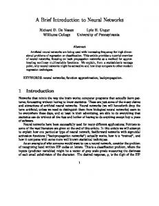
For real-valued functions f : Rn → R, the gradient ∇f (x) is a vector field. A vector field associates a vector to each point of (a subset of) Rn . In the case of the gradient vector field, every point a is given the vector ∇f (a), which points to the direction of greatest rate increase in the scalar field. (The scalar field associates a scalar value f (x) to each point x in Rn . In physics, common scalar fields are “temperature” in space, “pressure” in a fluid) The magnitude of ∇f (x) is the largest rate of increase. Figure 1.4 gives an illustration of the gradient vector field of the function f (x, y) = −(cos2 x+cos2 y)2 (taken from Wikipedia). The fact that ∇f (a) is the rate of increase is not hard to see. Recall that, for any direction v, the rate of increase of f along direction v is the directional derivative Dv f (a). As we have shown above in (2), Dv f (a) = dfa (v) = h∇f (a), vi ≤ k∇f (a)kkvk. Equality holds iff v is collinear with ∇f (a). Furthermore, the rate of increase is non-negative if v points to the same direction as ∇f (a). The level set corresponding to c ∈ R is the set of all points x ∈ Rn for which f (x) = c. When n = 2, we typically have level curves. When n = 3, we get level surfaces. For n > 3, level sets are typically level hypersurfaces. Proposition 1.6. When f is differentiable, ∇f (a) is perpendicular to the level set Sc corresponding to c = f (a). TBD: add a figure. Consider a smooth curve h : R → Rn passing through a in Sc , namely h is differentiable in a neighborhood of a, h(0) = a, and f (h(t)) = c for t sufficiently close to 0. Define (in a neighborhood of 0) a function g such that g(t) = f (h(t)). Then g 0 (0) = 0 obviously. By the chain rule, we also get 0 = g 0 (0) = h∇f (h(0)), h0 (0)i = h∇f (a), h0 (0)i. Hence, ∇f (a) is orthogonal to h0 (0) and thus it is orthogonal to the curve h. As h is arbitrary, ∇f (a) is orthogonal to the level set Sc . 5

Figure 1: The gradient of the function f (x, y) = −(cos2 x + cos2 y)2 depicted as a vector field on the bottom plane.

1.5

Taylor’s formula for multivariate functions

The basic idea of Taylor’s formula is to approximate f : Rn → R by a polynomial. The “error” term of this approximation can be written in several different ways, leading to different versions of the expansion. Recall that f is a class C k function if all the partial derivatives Di1 · · · Diq f exist and are continuous for any sequence i1 , · · · , iq where q ≤ k. In this case, it turns out that the order in which we take the partial derivatives is not important. For each r ∈ [n], let jr be the number of times that r appears in the sequence i1 , · · · , iq , then we can write Di1 · · · Diq f = D1j1 · · · Dnjn f =

∂ j1 f ∂xj11

···

∂ jn f ∂xjnn

.

If f is a class C k function, then for any j1 + · · · + jn ≤ k, the function D1j1 · · · Dnjn f is continuously differentiable. This means, for any non-zero vector h ∈ Rn , the directional derivative Dh D1j1 · · · Dnjn f exists. From (4), we can write Dh D1j1

· · · Dnjn f

=

n X

hi Di D1j1

· · · Dnjn f

i=1

=

n X i=1

6

hi D1j1 · · · Diji +1 · · · Dnjn f.

We can expand the above iteratively to obtain Dhk f

:= (h1 D1 + · · · + hn Dn )k f   X k hj1 · · · hjnn D1j1 · · · Dnjn f = j1 , · · · , jn 1 j1 +···+jn =k   X ∂ j1 f k ∂ jn f hj11 · · · hjnn j1 · · · jn . = j1 , · · · , jn ∂x1 ∂xn j1 +···+jn =k

The formula is notationally cumbersome. It is more common to use the multi-index notations: j = (j1 , · · · , jn )

(10)

|j| = j1 + · · · + jn

(11)

h

j

hj11 · · · hjnn D1j1 · · · Dnjn ∂f jn ∂f j1

=

Dj = ∂jf

=

xj

∂xj11

···

∂xjnn

(12) (13) .

(14)

Then, we can simplify the above formula as Dhk f =

X

Dj f =

|j|=k

X ∂jf . ∂xj

|j|=k

Theorem 1.7. Define Pk (h) =

k X Dr (a) h

r=1

r!

.

(15)

and Rk (h) = f (a + h) − Pk (h).

(16)

If f is a real-valued function of class C k+1 on an open set containing the line segment from a to a + h, then there exists ξ on the line segment such that Rk (h) =

Dhk+1 f (ξ) . (k + 1)!

(17)

In particular, f (a + h) =

k X Dr (a) h

r=0

r!

+

Dhk+1 f (ξ) . (k + 1)!

(18)

Furthermore, we have lim

h→0

Rk (h) = 0. khk

Of particular importance are the linear (k = 1) and quadratic case (k = 2). We state them separately. When k = 1, recall from (6) that Dh1 f (a) = ∇f (a)T h. 7

Corollary 1.8 (Linear Taylor Approximation). Suppose Ω ⊆ Rn is open, and f : Ω → R is differentiable, then f (a + h) = f (a) + ∇f (a)T h + o(|h|) as h → 0. (19) If f ∈ C 2 , then a stronger condition holds f (a + h) = f (a) + ∇f (a)T h + O(|h|2 ) as h → 0.

(20)

When k = 2 we can expand Dh2 f (a) = (h1 D1 + · · · + hn Dn )2 f (a) X = hi hj Di Dj f (a) i,j

= hT ∇2 f (a)h. Where, ∇2 f is the symmetric Hessian matrix ∂2f 2  ∂∂x2 f1   ∂x1 ∂x2

 ∇2 f := (Di Dj f )i,j =   

.. .

∂2f ∂x1 ∂xn

∂2f ∂x2 ∂x1 ∂2f ∂x22

.. .

∂2f ∂x2 ∂xn

··· ···

∂2f ∂xn ∂x1  ∂2f  ∂xn ∂x2 

··· ···



.. .

∂2f ∂x2n

  

(21)

Corollary 1.9 (Quadratic Taylor Approximation). Suppose Ω ⊆ Rn is open, and f : Ω → R is in C 2 , then 1 f (a + h) = f (a) + ∇f (a)T h + hT ∇2 f (a)h + o(|h|2 ) as h → 0. 2

(22)

If f ∈ C 3 , then a stronger condition holds 1 f (a + h) = f (a) + ∇f (a)T h + hT ∇2 f (a)h + O(|h|3 ) as h → 0. 2

2

(23)

Optimality conditions for unconstrained optimization

The basic ideas for these optimality conditions are very simple. However, carrying out the proof to every single technical detail could be tedious. We know from the previous section that we can approximate f at some point x∗ well. The linear expansion gives f (x∗ + h) − f (x∗ ) ≈ ∇f (x∗ )T h. Thus, if x∗ is an unconstrained local minimum of f , then for any sufficiently small variation h we have 0 ≤ f (x∗ + h) − f (x∗ ) ≈ ∇f (x∗ )T h. By replacing h with −h, we conclude that ∇f (x∗ )T h = 0 for all h, which means ∇f (x∗ ) = 0

8

is necessary for x∗ to be a local minimum (or maximum). The points x∗ for which ∇f (x∗ ) = 0 are called stationary points or critical points of f . (This necessary condition was formulated by Fermat in 1637 in the short treatise “Methodus as Disquirendam Maximam et Minimam” without proof (of course!).) Up to second order, we have a cost variation of 1 f (x∗ + h) − f (x∗ ) ≈ ∇f (x∗ )T h + hT ∇2 f (x∗ )h. 2 By the same reasoning, it must hold that hT ∇2 f (x∗ )h ≥ 0 for all small variations h. Thus, the Hessian must be positive semidefinite at local min/max-ima. Theorem 2.1 (Necessary Optimality Condition). Let x∗ be an unconstrained local minimum of f : Rn → R, and suppose f is continuously differentiable in an open set S containing x∗ . Then, ∇f (x∗ ) = 0

[First Order Necessary Condition]

(24)

If f is also twice continuously differentiable in S, then ∇2 f (x∗ ) is positive semidefinite.

[Second Order Necessary Condition]

(25)

Theorem 2.2 (Second Order Sufficient Optimality Condition). Let f : Rn → R be twice continuously differentiable in an open set S containing x∗ . Suppose x∗ satisfies the following: ∇f (x∗ ) = 0 and ∇2 f (x∗ ) is positive definite.

(26)

Then, x∗ is a strict unconstrained local minimum of f . (If “positive definite” is replaced by “negative definite” then x∗ is a strict unconstrained local maximum.)

3

Optimality conditions for constrained optimization

We further fix notations from multivariate calculus. Let f : Rn → Rm be a differentiable function with differentiable components f1 , · · · , fm . The gradient matrix of f , denoted by ∇f , is the n × m matrix whose jth column is the gradient of fj . Specifically,   ∇f (x) = ∇f1 (x) · · · ∇fm (x) . (Thus, the Jacobian of f is the transpose of ∇f .) If f : Rm+n → R is a function f (x, y) with x ∈ Rm and y ∈ Rn , then we define     ∂f (x,y) ∂y1

∂f (x,y) ∂x1

 ∇x f (x, y) =   ∇2x,x f (x, y) = ∇2x,y f (x, y) ∇2x,y f (y, y)

∂f (x,y) ∂xm  2  ∂ f (x, y)

∂xi ∂xj 

=  =

.. .

  

 ∇y f (x, y) =  

.. .

∂f (x,y) ∂yn

  

(note that this is a matrix)

ij

∂ 2 f (x, y) ∂xi ∂yj



∂ 2 f (x, y) ∂yi ∂yj



9

(note that this is a matrix) ij

(note that this is a matrix) ij

3.1

Lagrange multipliers and conditions for equality constraints

We consider optimization problems of the form min

f (x) h(x) = 0,

subject to

where f : Rn → R and h : Rn → Rm are continuously differentiable functions. Let the component functions of h be h1 , · · · , hm , then there are in fact m equality constraints hi (x) = 0, i ∈ [m]. The Lagrange multiplier theorem roughly relies on the following idea. Let S = {x | h(x) = 0} be the “surface” defined by h. If S is sufficiently “smooth” near x∗ , then it will have a “good” tangent space at x∗ . A tangent space at x∗ can be defined to be the space spanned by all tangent vectors at x∗ to curves passing through x∗ on S. Or, because the gradients ∇hi (x∗ ) are orthogonal to these curves, we can define the tangent space to be the span of all vectors orthogonal to all the ∇hi (x∗ ). Specifically,   V (x∗ ) := y | ∇hi (x∗ )T y = 0, ∀i ∈ [m] = y | h0 (x∗ )y = 0 . (27) A point x is said to be a regular point if the gradients ∇h1 (x), · · · , ∇hm (x) are linearly independent. We can show using the implicit function theorem that, if x∗ is regular then V (x∗ ) consists of all vectors which are tangent to some curves in S passing through x∗ . For x∗ to be a local extremum of f , the gradient ∇f (x∗ ) should be orthogonal to the tangent space V (x∗ ) (otherwise following some projection of ∇f (x∗ ) on the surface we should get an improvement on the objective). In other words, the objective gradient ∇f (x∗ ) must in the span of the constraint gradients ∇hi (x∗ ). Theorem 3.1 (Lagrange Multiplier Theorem – Necessary conditions). Let x∗ be a local minimum of f subject to h(x) = 0 such that x∗ is regular. Then, there exists a unique vector λ∗ = (λ∗1 , · · · , λ∗m ), called the Lagrange multiplier vector, such that ∇f (x∗ ) +

m X

λ∗i ∇hi (x∗ ) = 0.

(28)

i=1

If f and h are twice continuously differentiable, we also have the second order necessary condition ! m X yT ∇2 f (x∗ ) + λ∗i ∇2 hi (x∗ ) y ≥ 0, for all y ∈ V (x∗ )

(29)

i=1

where V (x∗ ) is the tangent space, which is also called the subspace of first order feasible variation: V (x∗ ) = {y | ∇hi (x∗ )T y = 0, i ∈ [m]}. The second order necessary condition can be shown by applying quadratic Taylor expansion of f . Now, define the Lagrangian function L : Rn+m → R by L(x, λ) = f (x) +

m X

λi hi (x).

(30)

i=1

Then, the first and second order necessary conditions above can be written by ∇x L(x∗ , λ∗ ) = 0, ∇λ L(x∗ , λ∗ ) = 0 10

(31)

(∇λ L(x∗ , λ∗ ) = 0 is the same as h(x∗ ) = 0), and yT ∇2x,x L(x∗ , λ∗ )y ≥ 0, for all y ∈ V (x∗ ).

(32)

Theorem 3.2 (Second Order Sufficiency Conditions). Suppose f and h are twice continuously differentiable. Suppose x∗ ∈ Rn and λ∗ ∈ Rm satisfy ∇x L(x∗ , λ∗ ) = 0, ∇λ L(x∗ , λ∗ ) = 0,

(33)

yT ∇2x,x L(x∗ , λ∗ )y > 0, for all y 6= 0, h0 (x∗ )y = 0.

(34)

and x∗

Then, is a strict local minimum of f subject to h(x) = 0. (If the positive definite condition is replaced by negative definite, then we get a strict local maximum.)

3.2

Karush-Kuhn-Tucker conditions for inequality constraints

We consider optimization problems of the form min subject to

f (x) h1 (x) = · · · = hm (x) = 0 g1 (x) ≤ 0, · · · , gr (x) ≤ 0,

where f, hi , gj are continuously differentiable functions from Rn to R. As usual, we can shorten the notations to min subject to

f (x) h(x) = 0, g(x) ≤ 0.

For a feasible point x, define the set of active constraints at x to be A(x) = {j | gj (x) = 0}.

(35)

The feasible point x is said to be regular if the equality constraint gradients hi (x), i ∈ [m] and the inactive constraint gradients gj (x), j ∈ A(x) are linearly independent. (If there’s no equality constraint, and all inequality constraints are inactive, then x is also called “regular.”) The Lagrangian function in this case is defined to be m r X X L(x, λ, µ) = f (x) + λi hi (x) + µj gj (x). (36) i=1

j=1

Theorem 3.3 (KKT Necessary Conditions). Let x∗ be a regular local minimum of the problem min subject to

f (x) h(x) = 0, g(x) ≤ 0,

where f, hi , gj are continuously differentiable. Then there exist λ∗ ∈ Rm , µ∗ ∈ Rr , such that ∇x L(x∗ , λ∗ , µ∗ ) = 0, µ∗j ≥ 0, j ∈ [r], µ∗j = 0, ∀j ∈ / A(x∗ ). 11

In addition, if f, g, h are twice continuously differentiable, then yT ∇2x,x L(x∗ , λ∗ , µ∗ )y ≥ 0, for all y ∈ Rn such that ∇hi (x∗ )T y = 0, ∀i ∈ [m] and ∇gj (x∗ )T y = 0, ∀j ∈ A(x∗ ). Theorem 3.4 (Second Order Sufficiency Conditions). Let f, g, h be twice continuously differentiable. Suppose x∗ , λ∗ , µ∗ satisfy ∇x L(x∗ , λ∗ , µ∗ ) = 0, h(x∗ ) = 0, g(x∗ ) ≤ 0, µ∗j ≥ 0, j ∈ [r] µ∗j = 0, j ∈ / A(x∗ ) and yT ∇2x,x L(x∗ , λ∗ , µ∗ )y > 0 for all 0 6= y ∈ Rn such that ∇hi (x∗ )T y = 0, ∀i ∈ [m] and ∇gj (x∗ )T y = 0, ∀j ∈ A(x∗ ). Assume also that µ∗j > 0, ∀j ∈ A(x∗ ). (This is known as the strict complementary slackness condition.) Then, x∗ is a strict local minimum of f subject to h(x) = 0, g(x) ≤ 0.

References [1] D. P. B ERTSEKAS AND D. P. B ERTSEKAS, Nonlinear Programming, Athena Scientific, 2nd ed., September 1999. [2] S. B OYD AND L. VANDENBERGHE, Convex optimization, Cambridge University Press, Cambridge, 2004. ´ [3] V. C HV ATAL , Linear programming, A Series of Books in the Mathematical Sciences, W. H. Freeman and Company, New York, 1983. [4] C. H. E DWARDS , J R ., Advanced calculus of several variables, Dover Publications Inc., New York, 1994. Corrected reprint of the 1973 original. [5] A. S CHRIJVER, Theory of linear and integer programming, Wiley-Interscience Series in Discrete Mathematics, John Wiley & Sons Ltd., Chichester, 1986. A Wiley-Interscience Publication. [6] G. S TRANG, Linear algebra and its applications, Academic Press [Harcourt Brace Jovanovich Publishers], New York, second ed., 1980.

12