3.2.1 A simple proof of Kuhn-Tucker conditions for equality constraints . ...... Such a point is called a saddle point (see Figure 2.2 for a geometrical illustration). If xâ is a stationary point and â2 f(xâ) is semi-definite it is not possible to draw any.
OPTIMIZATION An introduction A. Astolfi First draft – September 2002 Last revision – September 2006
Contents 1 Introduction 1.1 Introduction . . . . . . . . . . . . . . . 1.2 Statement of an optimization problem 1.2.1 Design vector . . . . . . . . . . 1.2.2 Design constraints . . . . . . . 1.2.3 Objective function . . . . . . . 1.3 Classification of optimization problems 1.4 Examples . . . . . . . . . . . . . . . .
. . . . . . .
. . . . . . .
. . . . . . .
. . . . . . .
. . . . . . .
. . . . . . .
. . . . . . .
. . . . . . .
. . . . . . .
2 Unconstrained optimization 2.1 Introduction . . . . . . . . . . . . . . . . . . . . . . . . 2.2 Definitions and existence conditions . . . . . . . . . . 2.3 General properties of minimization algorithms . . . . . 2.3.1 General unconstrained minimization algorithm 2.3.2 Existence of accumulation points . . . . . . . . 2.3.3 Condition of angle . . . . . . . . . . . . . . . . 2.3.4 Speed of convergence . . . . . . . . . . . . . . . 2.4 Line search . . . . . . . . . . . . . . . . . . . . . . . . 2.4.1 Exact line search . . . . . . . . . . . . . . . . . 2.4.2 Armijo method . . . . . . . . . . . . . . . . . . 2.4.3 Goldstein conditions . . . . . . . . . . . . . . . 2.4.4 Line search without derivatives . . . . . . . . . 2.4.5 Implementation of a line search algorithm . . . 2.5 The gradient method . . . . . . . . . . . . . . . . . . . 2.6 Newton’s method . . . . . . . . . . . . . . . . . . . . . 2.6.1 Method of the trust region . . . . . . . . . . . 2.6.2 Non-monotonic line search . . . . . . . . . . . . 2.6.3 Comparison between Newton’s method and the 2.7 Conjugate directions methods . . . . . . . . . . . . . . 2.7.1 Modification of βk . . . . . . . . . . . . . . . . 2.7.2 Modification of αk . . . . . . . . . . . . . . . . 2.7.3 Polak-Ribiere algorithm . . . . . . . . . . . . . 2.8 Quasi-Newton methods . . . . . . . . . . . . . . . . . iii
. . . . . . .
. . . . . . .
. . . . . . .
. . . . . . .
. . . . . . .
. . . . . . . . . . . . . . . . . . . . . . . . . . . . . . . . . . . . . . . . . . . . . . . . . . . . . . . . . . . . . . . . . . . . . . . . . . . . . . . . . . . . . gradient . . . . . . . . . . . . . . . . . . . . . . . . .
. . . . . . .
. . . . . . .
. . . . . . .
1 2 3 4 4 4 6 6
. . . . . . . . . . . . . . . . . . . . . . . . . . . . . . . . . . . . . . . . . . . . . . . . . . . . . . . . . . . . . . . . . . . . . . . . . . . . . . . . . . . . . method . . . . . . . . . . . . . . . . . . . . . . . . .
. . . . . . . . . . . . . . . . . . . . . . .
. . . . . . . . . . . . . . . . . . . . . . .
9 10 10 17 17 18 19 22 23 24 24 26 27 29 29 31 35 36 37 37 40 41 41 42
. . . . . . .
. . . . . . .
. . . . . . .
. . . . . . .
CONTENTS
iv 2.9
Methods without derivatives . . . . . . . . . . . . . . . . . . . . . . . . . . . 45
3 Nonlinear programming 3.1 Introduction . . . . . . . . . . . . . . . . . . . . . . . . . . . . . . . . . . . 3.2 Definitions and existence conditions . . . . . . . . . . . . . . . . . . . . . 3.2.1 A simple proof of Kuhn-Tucker conditions for equality constraints 3.2.2 Quadratic cost function with linear equality constraints . . . . . . 3.3 Nonlinear programming methods: introduction . . . . . . . . . . . . . . . 3.4 Sequential and exact methods . . . . . . . . . . . . . . . . . . . . . . . . . 3.4.1 Sequential penalty functions . . . . . . . . . . . . . . . . . . . . . . 3.4.2 Sequential augmented Lagrangian functions . . . . . . . . . . . . . 3.4.3 Exact penalty functions . . . . . . . . . . . . . . . . . . . . . . . . 3.4.4 Exact augmented Lagrangian functions . . . . . . . . . . . . . . . 3.5 Recursive quadratic programming . . . . . . . . . . . . . . . . . . . . . . . 3.6 Concluding remarks . . . . . . . . . . . . . . . . . . . . . . . . . . . . . .
. . . . . . . . . . . .
49 50 51 53 54 54 55 55 57 59 61 62 64
4 Global optimization 4.1 Introduction . . . . . . . . . . . . . . . . 4.2 Deterministic methods . . . . . . . . . . 4.2.1 Methods for Lipschitz functions . 4.2.2 Methods of the trajectories . . . 4.2.3 Tunneling methods . . . . . . . . 4.3 Probabilistic methods . . . . . . . . . . 4.3.1 Methods using random directions 4.3.2 Multistart methods . . . . . . . . 4.3.3 Stopping criteria . . . . . . . . .
. . . . . . . . .
65 66 66 66 68 70 71 71 72 72
. . . . . . . . .
. . . . . . . . .
. . . . . . . . .
. . . . . . . . .
. . . . . . . . .
. . . . . . . . .
. . . . . . . . .
. . . . . . . . .
. . . . . . . . .
. . . . . . . . .
. . . . . . . . .
. . . . . . . . .
. . . . . . . . .
. . . . . . . . .
. . . . . . . . .
. . . . . . . . .
. . . . . . . . .
. . . . . . . . .
. . . . . . . . .
List of Figures 1.1 1.2 1.3 2.1 2.2 2.3 2.4 2.5 2.6 2.7
4.1 4.2 4.3 4.4
Feasible region in a two-dimensional design space. Only inequality straints are present. . . . . . . . . . . . . . . . . . . . . . . . . . . . Design space, objective functions surfaces, and optimum point. . . . Electrical bridge network. . . . . . . . . . . . . . . . . . . . . . . . .
con. . . . . . . . . . . .
Geometrical interpretation of the anti-gradient. . . . . . . . . . . . . . . . A saddle point in IR2 . . . . . . . . . . . . . . . . . . . . . . . . . . . . . . Geometrical interpretation of Armijo method. . . . . . . . . . . . . . . . . Geometrical interpretation of Goldstein method. . . . . . . . . . . . . . . � ξ−1 . . . . . . . . . . . . . . . . . . . . . . . . . . . . . The function ξ ξ+1 Behavior of the gradient algorithm. . . . . . . . . . . . . . . . . . . . . . . The simplex method. The points x(1) , x(2) and x(3) yields the starting simplex. The second simplex is given by the points x(1) , x(2) and x(4) . The third simplex is given by the points x(2) , x(4) and x(5) . . . . . . . . . . . .
. 47
Geometrical interpretation of the Lipschitz conditions (4.2) and Geometrical interpretation of Schubert-Mladineo algorithm. . . Interpretation of the tunneling phase. . . . . . . . . . . . . . . The functions f (x) and T (x, x�k ). . . . . . . . . . . . . . . . . .
. . . .
v
(4.3). . . . . . . . . . . . .
. . . .
. . . .
. . . .
4 5 6 13 16 25 27
. 30 . 31
66 68 70 71
vi
LIST OF FIGURES
List of Tables 1.1
Properties of the articles to load. . . . . . . . . . . . . . . . . . . . . . . . .
2.1
Comparison between the gradient method and Newton’s method. . . . . . . 37
vii
7
viii
LIST OF TABLES
Chapter 1
Introduction
CHAPTER 1. INTRODUCTION
2
1.1
Introduction
Optimization is the act of achieving the best possible result under given circumstances. In design, construction, maintenance, ..., engineers have to take decisions. The goal of all such decisions is either to minimize effort or to maximize benefit. The effort or the benefit can be usually expressed as a function of certain design variables. Hence, optimization is the process of finding the conditions that give the maximum or the minimum value of a function. It is obvious that if a point x� corresponds to the minimum value of a function f (x), the same point corresponds to the maximum value of the function −f (x). Thus, optimization can be taken to be minimization. There is no single method available for solving all optimization problems efficiently. Hence, a number of methods have been developed for solving different types of problems. Optimum seeking methods are also known as mathematical programming techniques, which are a branch of operations research. Operations research is coarsely composed of the following areas. • Mathematical programming methods. These are useful in finding the minimum of a function of several variables under a prescribed set of constraints. • Stochastic process techniques. These are used to analyze problems which are described by a set of random variables of known distribution. • Statistical methods. These are used in the analysis of experimental data and in the construction of empirical models. These lecture notes deal mainly with the theory and applications of mathematical programming methods. Mathematical programming is a vast area of mathematics and engineering. It includes • calculus of variations and optimal control; • linear, quadratic and non-linear programming; • geometric programming; • integer programming; • network methods (PERT); • game theory. The existence of optimization can be traced back to Newton, Lagrange and Cauchy. The development of differential methods for optimization was possible because of the contribution of Newton and Leibnitz. The foundations of the calculus of variations were laid by Bernoulli, Euler, Lagrange and Weierstrasse. Constrained optimization was first studied by Lagrange and the notion of descent was introduced by Cauchy.
1.2. STATEMENT OF AN OPTIMIZATION PROBLEM
3
Despite these early contributions, very little progress was made till the 20th century, when computer power made the implementation of optimization procedures possible and this in turn stimulated further research methods. The major developments in the area of numerical methods for unconstrained optimization have been made in the UK. These include the development of the simplex method (Dantzig, 1947), the principle of optimality (Bellman, 1957), necessary and sufficient conditions of optimality (Kuhn and Tucker, 1951). Optimization in its broadest sense can be applied to solve any engineering problem, e.g. • design of aircraft for minimum weight; • optimal (minimum time) trajectories for space missions; • minimum weight design of structures for earthquake; • optimal design of electric networks; • optimal production planning, resources allocation, scheduling; • shortest route; • design of optimum pipeline networks; • minimum processing time in production systems; • optimal control.
1.2
Statement of an optimization problem
An optimization, or a mathematical programming problem can be stated as follows. Find x = (x1 , x2 , ...., xn ) which minimizes f (x) subject to the constraints gj (x) ≤ 0
(1.1)
lj (x) = 0
(1.2)
for j = 1, . . . , m, and for j = 1, . . . , p. The variable x is called the design vector, f (x) is the objective function, gj (x) are the inequality constraints and lj (x) are the equality constraints. The number of variables n and the number of constraints p + m need not be related. If p + m = 0 the problem is called an unconstrained optimization problem.
CHAPTER 1. INTRODUCTION
4
g4 = 0
x2
xxxxxxxxxxxxxxxxxxxxxxxxxxxxxxxxxxxxxxxxxxxxxxxxxxxxxxxxxxxxxxxxxxxxxxxxxxxxxxxxxxxxxxxxx xxxxxxxxxxxxxxxxxxxxxxxxxxxxxxxxxxxxxxxxxxxxxxxxxxxxxxxxxxxxxxxxxxxxxxxxxxxxxxxxxxxxxxxxx xxxxxxxxxxxxxxxxxxxxxxxxxxxxxxxxxxxxxxxxxxxxxxxxxxxxxxxxxxxxxxxxxxxxxxxxxxxxxxxxxxxxxxxxx xxxxxxxxxxxxxxxxxxxxxxxxxxxxxxxxxxxxxxxxxxxxxxxxxxxxxxxxxxxxxxxxxxxxxxxxxxxxxxxxxxxxxxxxx xxxxxxxxxxxxxxxxxxxxxxxxxxxxxxxxxxxxxxxxxxxxxxxxxxxxxxxxxxxxxxxxxxxxxxxxxxxxxxxxxxxxxxxxx xxxxxxxxxxxxxxxxxxxxxxxxxxxxxxxxxxxxxxxxxxxxxxxxxxxxxxxxxxxxxxxxxxxxxxxxxxxxxxxxxxxxxxxxx xxxxxxxxxxxxxxxxxxxxxxxxxxxxxxxxxxxxxxxxxxxxxxxxxxxxxxxxxxxxxxxxxxxxxxxxxxxxxxxxxxxxxxxxx xxxxxxxxxxxxxxxxxxxxxxxxxxxxxxxxxxxxxxxxxxxxxxxxxxxxxxxxxxxxxxxxxxxxxxxxxxxxxxxxxxxxxxxxx xxxxxxxxxxxxxxxxxxxxxxxxxxxxxxxxxxxxxxxxxxxxxxxxxxxxxxxxxxxxxxxxxxxxxxxxxxxxxxxxxxxxxxxxx xxxxxxxxxxxxxxxxxxxxxxxxxxxxxxxxxxxxxxxxxxxxxxxxxxxxxxxxxxxxxxxxxxxxxxxxxxxxxxxxxxxxxxxxx xxxxxxxxxxxxxxxxxxxxxxxxxxxxxxxxxxxxxxxxxxxxxxxxxxxxxxxxxxxxxxxxxxxxxxxxxxxxxxxxxxxxxxxxx xxxxxxxxxxxxxxxxxxxxxxxxxxxxxxxxxxxxxxxxxxxxxxxxxxxxxxxxxxxxxxxxxxxxxxxxxxxxxxxxxxxxxxxxx xxxxxxxxxxxxxxxxxxxxxxxxxxxxxxxxxxxxxxxxxxxxxxxxxxxxxxxxxxxxxxxxxxxxxxxxxxxxxxxxxxxxxxxxx xxxxxxxxxxxxxxxxxxxxxxxxxxxxxxxxxxxxxxxxxxxxxxxxxxxxxxxxxxxxxxxxxxxxxxxxxxxxxxxxxxxxxxxxx xxxxxxxxxxxxxxxxxxxxxxxxxxxxxxxxxxxxxxxxxxxxxxxxxxxxxxxxxxxxxxxxxxxxxxxxxxxxxxxxxxxxxxxxx xxxxxxxxxxxxxxxxxxxxxxxxxxxxxxxxxxxxxxxxxxxxxxxxxxxxxxxxxxxxxxxxxxxxxxxxxxxxxxxxxxxxxxxxx xxxxxxxxxxxxxxxxxxxxxxxxxxxxxxxxxxxxxxxxxxxxxxxxxxxxxxxxxxxxxxxxxxxxxxxxxxxxxxxxxxxxxxxxx xxxxxxxxxxxxxxxxxxxxxxxxxxxxxxxxxxxxxxxxxxxxxxxxxxxxxxxxxxxxxxxxxxxxxxxxxxxxxxxxxxxxxxxxx xxxxxxxxxxxxxxxxxxxxxxxxxxxxxxxxxxxxxxxxxxxxxxxxxxxxxxxxxxxxxxxxxxxxxxxxxxxxxxxxxxxxxxxxx xxxxxxxxxxxxxxxxxxxxxxxxxxxxxxxxxxxxxxxxxxxxxxxxxxxxxxxxxxxxxxxxxxxxxxxxxxxxxxxxxxxxxxxxx xxxxxxxxxxxxxxxxxxxxxxxxxxxxxxxxxxxxxxxxxxxxxxxxxxxxxxxxxxxxxxxxxxxxxxxxxxxxxxxxxxxxxxxxx xxxxxxxxxxxxxxxxxxxxxxxxxxxxxxxxxxxxxxxxxxxxxxxxxxxxxxxxxxxxxxxxxxxxxxxxxxxxxxxxxxxxxxxxx xxxxxxxxxxxxxxxxxxxxxxxxxxxxxxxxxxxxxxxxxxxxxxxxxxxxxxxxxxxxxxxxxxxxxxxxxxxxxxxxxxxxxxxxx xxxxxxxxxxxxxxxxxxxxxxxxxxxxxxxxxxxxxxxxxxxxxxxxxxxxxxxxxxxxxxxxxxxxxxxxxxxxxxxxxxxxxxxxx xxxxxxxxxxxxxxxxxxxxxxxxxxxxxxxxxxxxxxxxxxxxxxxxxxxxxxxxxxxxxxxxxxxxxxxxxxxxxxxxxxxxxxxxx xxxxxxxxxxxxxxxxxxxxxxxxxxxxxxxxxxxxxxxxxxxxxxxxxxxxxxxxxxxxxxxxxxxxxxxxxxxxxxxxxxxxxxxxx xxxxxxxxxxxxxxxxxxxxxxxxxxxxxxxxxxxxxxxxxxxxxxxxxxxxxxxxxxxxxxxxxxxxxxxxxxxxxxxxxxxxxxxxx xxxxxxxxxxxxxxxxxxxxxxxxxxxxxxxxxxxxxxxxxxxxxxxxxxxxxxxxxxxxxxxxxxxxxxxxxxxxxxxxxxxxxxxxx xxxxxxxxxxxxxxxxxxxxxxxxxxxxxxxxxxxxxxxxxxxxxxxxxxxxxxxxxxxxxxxxxxxxxxxxxxxxxxxxxxxxxxxxx xxxxxxxxxxxxxxxxxxxxxxxxxxxxxxxxxxxxxxxxxxxxxxxxxxxxxxxxxxxxxxxxxxxxxxxxxxxxxxxxxxxxxxxxx xxxxxxxxxxxxxxxxxxxxxxxxxxxxxxxxxxxxxxxxxxxxxxxxxxxxxxxxxxxxxxxxxxxxxxxxxxxxxxxxxxxxxxxxx xxxxxxxxxxxxxxxxxxxxxxxxxxxxxxxxxxxxxxxxxxxxxxxxxxxxxxxxxxxxxxxxxxxxxxxxxxxxxxxxxxxxxxxxx xxxxxxxxxxxxxxxxxxxxxxxxxxxxxxxxxxxxxxxxxxxxxxxxxxxxxxxxxxxxxxxxxxxxxxxxxxxxxxxxxxxxxxxxx xxxxxxxxxxxxxxxxxxxxxxxxxxxxxxxxxxxxxxxxxxxxxxxxxxxxxxxxxxxxxxxxxxxxxxxxxxxxxxxxxxxxxxxxx xxxxxxxxxxxxxxxxxxxxxxxxxxxxxxxxxxxxxxxxxxxxxxxxxxxxxxxxxxxxxxxxxxxxxxxxxxxxxxxxxxxxxxxxx xxxxxxxxxxxxxxxxxxxxxxxxxxxxxxxxxxxxxxxxxxxxxxxxxxxxxxxxxxxxxxxxxxxxxxxxxxxxxxxxxxxxxxxxx xxxxxxxxxxxxxxxxxxxxxxxxxxxxxxxxxxxxxxxxxxxxxxxxxxxxxxxxxxxxxxxxxxxxxxxxxxxxxxxxxxxxxxxxx xxxxxxxxxxxxxxxxxxxxxxxxxxxxxxxxxxxxxxxxxxxxxxxxxxxxxxxxxxxxxxxxxxxxxxxxxxxxxxxxxxxxxxxxx xxxxxxxxxxxxxxxxxxxxxxxxxxxxxxxxxxxxxxxxxxxxxxxxxxxxxxxxxxxxxxxxxxxxxxxxxxxxxxxxxxxxxxxxx xxxxxxxxxxxxxxxxxxxxxxxxxxxxxxxxxxxxxxxxxxxxxxxxxxxxxxxxxxxxxxxxxxxxxxxxxxxxxxxxxxxxxxxxx xxxxxxxxxxxxxxxxxxxxxxxxxxxxxxxxxxxxxxxxxxxxxxxxxxxxxxxxxxxxxxxxxxxxxxxxxxxxxxxxxxxxxxxxx xxxxxxxxxxxxxxxxxxxxxxxxxxxxxxxxxxxxxxxxxxxxxxxxxxxxxxxxxxxxxxxxxxxxxxxxxxxxxxxxxxxxxxxxx xxxxxxxxxxxxxxxxxxxxxxxxxxxxxxxxxxxxxxxxxxxxxxxxxxxxxxxxxxxxxxxxxxxxxxxxxxxxxxxxxxxxxxxxx xxxxxxxxxxxxxxxxxxxxxxxxxxxxxxxxxxxxxxxxxxxxxxxxxxxxxxxxxxxxxxxxxxxxxxxxxxxxxxxxxxxxxxxxx xxxxxxxxxxxxxxxxxxxxxxxxxxxxxxxxxxxxxxxxxxxxxxxxxxxxxxxxxxxxxxxxxxxxxxxxxxxxxxxxxxxxxxxxx xxxxxxxxxxxxxxxxxxxxxxxxxxxxxxxxxxxxxxxxxxxxxxxxxxxxxxxxxxxxxxxxxxxxxxxxxxxxxxxxxxxxxxxxx xxxxxxxxxxxxxxxxxxxxxxxxxxxxxxxxxxxxxxxxxxxxxxxxxxxxxxxxxxxxxxxxxxxxxxxxxxxxxxxxxxxxxxxxx xxxxxxxxxxxxxxxxxxxxxxxxxxxxxxxxxxxxxxxxxxxxxxxxxxxxxxxxxxxxxxxxxxxxxxxxxxxxxxxxxxxxxxxxx xxxxxxxxxxxxxxxxxxxxxxxxxxxxxxxxxxxxxxxxxxxxxxxxxxxxxxxxxxxxxxxxxxxxxxxxxxxxxxxxxxxxxxxxx xxxxxxxxxxxxxxxxxxxxxxxxxxxxxxxxxxxxxxxxxxxxxxxxxxxxxxxxxxxxxxxxxxxxxxxxxxxxxxxxxxxxxxxxx xxxxxxxxxxxxxxxxxxxxxxxxxxxxxxxxxxxxxxxxxxxxxxxxxxxxxxxxxxxxxxxxxxxxxxxxxxxxxxxxxxxxxxxxx xxxxxxxxxxxxxxxxxxxxxxxxxxxxxxxxxxxxxxxxxxxxxxxxxxxxxxxxxxxxxxxxxxxxxxxxxxxxxxxxxxxxxxxxx xxxxxxxxxxxxxxxxxxxxxxxxxxxxxxxxxxxxxxxxxxxxxxxxxxxxxxxxxxxxxxxxxxxxxxxxxxxxxxxxxxxxxxxxx xxxxxxxxxxxxxxxxxxxxxxxxxxxxxxxxxxxxxxxxxxxxxxxxxxxxxxxxxxxxxxxxxxxxxxxxxxxxxxxxxxxxxxxxx xxxxxxxxxxxxxxxxxxxxxxxxxxxxxxxxxxxxxxxxxxxxxxxxxxxxxxxxxxxxxxxxxxxxxxxxxxxxxxxxxxxxxxxxx xxxxxxxxxxxxxxxxxxxxxxxxxxxxxxxxxxxxxxxxxxxxxxxxxxxxxxxxxxxxxxxxxxxxxxxxxxxxxxxxxxxxxxxxx xxxxxxxxxxxxxxxxxxxxxxxxxxxxxxxxxxxxxxxxxxxxxxxxxxxxxxxxxxxxxxxxxxxxxxxxxxxxxxxxxxxxxxxxx xxxxxxxxxxxxxxxxxxxxxxxxxxxxxxxxxxxxxxxxxxxxxxxxxxxxxxxxxxxxxxxxxxxxxxxxxxxxxxxxxxxxxxxxx xxxxxxxxxxxxxxxxxxxxxxxxxxxxxxxxxxxxxxxxxxxxxxxxxxxxxxxxxxxxxxxxxxxxxxxxxxxxxxxxxxxxxxxxx xxxxxxxxxxxxxxxxxxxxxxxxxxxxxxxxxxxxxxxxxxxxxxxxxxxxxxxxxxxxxxxxxxxxxxxxxxxxxxxxxxxxxxxxx xxxxxxxxxxxxxxxxxxxxxxxxxxxxxxxxxxxxxxxxxxxxxxxxxxxxxxxxxxxxxxxxxxxxxxxxxxxxxxxxxxxxxxxxx xxxxxxxxxxxxxxxxxxxxxxxxxxxxxxxxxxxxxxxxxxxxxxxxxxxxxxxxxxxxxxxxxxxxxxxxxxxxxxxxxxxxxxxxx xxxxxxxxxxxxxxxxxxxxxxxxxxxxxxxxxxxxxxxxxxxxxxxxxxxxxxxxxxxxxxxxxxxxxxxxxxxxxxxxxxxxxxxxx xxxxxxxxxxxxxxxxxxxxxxxxxxxxxxxxxxxxxxxxxxxxxxxxxxxxxxxxxxxxxxxxxxxxxxxxxxxxxxxxxxxxxxxxx xxxxxxxxxxxxxxxxxxxxxxxxxxxxxxxxxxxxxxxxxxxxxxxxxxxxxxxxxxxxxxxxxxxxxxxxxxxxxxxxxxxxxxxxx xxxxxxxxxxxxxxxxxxxxxxxxxxxxxxxxxxxxxxxxxxxxxxxxxxxxxxxxxxxxxxxxxxxxxxxxxxxxxxxxxxxxxxxxx xxxxxxxxxxxxxxxxxxxxxxxxxxxxxxxxxxxxxxxxxxxxxxxxxxxxxxxxxxxxxxxxxxxxxxxxxxxxxxxxxxxxxxxxx xxxxxxxxxxxxxxxxxxxxxxxxxxxxxxxxxxxxxxxxxxxxxxxxxxxxxxxxxxxxxxxxxxxxxxxxxxxxxxxxxxxxxxxxx xxxxxxxxxxxxxxxxxxxxxxxxxxxxxxxxxxxxxxxxxxxxxxxxxxxxxxxxxxxxxxxxxxxxxxxxxxxxxxxxxxxxxxxxx xxxxxxxxxxxxxxxxxxxxxxxxxxxxxxxxxxxxxxxxxxxxxxxxxxxxxxxxxxxxxxxxxxxxxxxxxxxxxxxxxxxxxxxxx xxxxxxxxxxxxxxxxxxxxxxxxxxxxxxxxxxxxxxxxxxxxxxxxxxxxxxxxxxxxxxxxxxxxxxxxxxxxxxxxxxxxxxxxx xxxxxxxxxxxxxxxxxxxxxxxxxxxxxxxxxxxxxxxxxxxxxxxxxxxxxxxxxxxxxxxxxxxxxxxxxxxxxxxxxxxxxxxxx xxxxxxxxxxxxxxxxxxxxxxxxxxxxxxxxxxxxxxxxxxxxxxxxxxxxxxxxxxxxxxxxxxxxxxxxxxxxxxxxxxxxxxxxx xxxxxxxxxxxxxxxxxxxxxxxxxxxxxxxxxxxxxxxxxxxxxxxxxxxxxxxxxxxxxxxxxxxxxxxxxxxxxxxxxxxxxxxxx xxxxxxxxxxxxxxxxxxxxxxxxxxxxxxxxxxxxxxxxxxxxxxxxxxxxxxxxxxxxxxxxxxxxxxxxxxxxxxxxxxxxxxxxx xxxxxxxxxxxxxxxxxxxxxxxxxxxxxxxxxxxxxxxxxxxxxxxxxxxxxxxxxxxxxxxxxxxxxxxxxxxxxxxxxxxxxxxxx xxxxxxxxxxxxxxxxxxxxxxxxxxxxxxxxxxxxxxxxxxxxxxxxxxxxxxxxxxxxxxxxxxxxxxxxxxxxxxxxxxxxxxxxx
Infeasible region
Feasible region
g3 = 0
g1 = 0
g2 = 0
x1 Figure 1.1: Feasible region in a two-dimensional design space. Only inequality constraints are present.
1.2.1
Design vector
Any system is described by a set of quantities, some of which are viewed as variables during the design process, and some of which are preassigned parameters or are imposed by the environment. All the quantities that can be treated as variables are called design or decision variables, and are collected in the design vector x.
1.2.2
Design constraints
In practice, the design variables cannot be selected arbitrarily, but have to satisfy certain requirements. These restrictions are called design constraints. Design constraints may represent limitation on the performance or behaviour of the system or physical limitations. Consider, for example, an optimization problem with only inequality constraints, i.e. gj (x) ≤ 0. The set of values of x that satisfy the equations gj (x) = 0 forms a hypersurface in the design space, which is called constraint surface. In general, if n is the number of design variables, the constraint surface is an n − 1 dimensional surface. The constraint surface divides the design space into two regions: one in which gj (x) < 0 and one in which gj (x) > 0. The points x on the constraint surface satisfy the constraint critically, whereas the points x such that gj (x) > 0, for some j, are infeasible, i.e. are unacceptable, see Figure 1.1.
1.2.3
Objective function
The classical design procedure aims at finding an acceptable design, i.e. a design which satisfies the constraints. In general there are several acceptable designs, and the purpose
1.2. STATEMENT OF AN OPTIMIZATION PROBLEM
x2
5
Feasible region
f=d f=c f=b f=a
Optimum point
x1 a f (x0 ) ≥ f (x� ), hence x� is a global minimum � of f in IRn . It is obvious that the structure of the level sets of the function f plays a fundamental role in the solution of Problem 1. The following result provides a necessary and sufficient condition for the compactness of all level sets of f . 3
A compact set is a bounded and closed set.
CHAPTER 2. UNCONSTRAINED OPTIMIZATION
12
Proposition 3 Let f : IRn → IR be a continuous function. All level sets of f are compact if and only if for any sequence {xk } one has lim �xk � = ∞
k→∞
⇒
Remark. In general xk ∈ IRn , namely
⎡ ⎢ ⎢ xk = ⎢ ⎢ ⎣
lim f (xk ) = ∞.
k→∞
x1k x2k .. .
⎤ ⎥ ⎥ ⎥, ⎥ ⎦
xnk �
i.e. we use superscripts to denote components of a vector.
A function that satisfies the condition of the above proposition is said to be radially unbounded. Proof. We only prove the necessity. Suppose all level sets of f are compact. Then, proceeding by contradiction, suppose there exist a sequence {xk } such that limk→∞ �xk � = ∞ and a number γ > 0 such that f (xk ) ≤ γ < ∞ for all k. As a result {xk } ⊂ L(γ). However, by compactness of L(γ) it is not possible that limk→∞ �xk � = ∞.
�
Definition 4 Let f : IRn → IR. A vector d ∈ IRn is said to be a descent direction for f in x� if there exists δ > 0 such that f (x� + λd) < f (x� ), for all λ ∈ (0, δ). If the function f is differentiable it is possible to give a simple condition guaranteeing that a certain direction is a descent direction. Proposition 4 Let f : IRn → IR and assume4 ∇f exists and is continuous. Let x� and d be given. Then, if ∇f (x� )� d < 0 the direction d is a descent direction for f at x� . Proof. Note that ∇f (x� )� d is the directional derivative of f (which is differentiable by hypothesis) at x� along d, i.e. ∇f (x� )� d = lim
λ→0+
f (x� + λd) − f (x� ) , λ
∂f We denote with ∇f the gradient of the function f , i.e. ∇f = [ ∂x 1,···, column vector. 4
∂f � ]. ∂xn
Note that ∇f is a
2.2. DEFINITIONS AND EXISTENCE CONDITIONS
13
f increasing f(x) = f(x2) > f(x1) f(x) = f(x1) > f(x ) * f(x) = f(x *) anti-gradient descent direction Figure 2.1: Geometrical interpretation of the anti-gradient.
and this is negative by hypothesis. As a result, for λ > 0 and sufficiently small f (x� + λd) − f (x� ) < 0, hence the claim.
�
The proposition establishes that if ∇f (x� )� d < 0 then for sufficiently small positive displacements along d and starting at x� the function f is decreasing. It is also obvious that if ∇f (x� )� d > 0, d is a direction of ascent, i.e. the function f is increasing for sufficiently small positive displacements from x� along d. If ∇f (x� )� d = 0, d is orthogonal to ∇f (x� ) and it is not possible to establish, without further knowledge on the function f , what is the nature of the direction d. From a geometrical point of view (see also Figure 2.1), the sign of the directional derivative ∇f (x� )� d gives information on the angle between d and the direction of the gradient at x� , provided ∇f (x� ) �= 0. If ∇f (x� )� d > 0 the angle between ∇f (x� ) and d is acute. If ∇f (x� )� d < 0 the angle between ∇f (x� ) and d is obtuse. Finally, if ∇f (x� )� d = 0, and ∇f (x� ) �= 0, ∇f (x� ) and d are orthogonal. Note that the gradient ∇f (x� ), if it is not identically zero, is a direction orthogonal to the level surface {x : f (x) = f (x� )} and it is a direction of ascent, hence the anti-gradient −∇f (x� ) is a descent direction. Remark. The scalar product x� y between the two vectors x and y can be used to define the angle between x and y. For, define the angle between x and y as the number θ ∈ [0, π] such that5 x� y cos θ = . �x�E �y�E If x� y = 0 one has cos θ = 0 and the vectors are orthogonal, whereas if x and y have the same direction, i.e. x = λy with λ > 0, cos θ = 1. � 5
�x�E denotes the Euclidean norm of the the vector x, i.e. �x�E =
√
x� x.
CHAPTER 2. UNCONSTRAINED OPTIMIZATION
14
We are now ready to state and prove some necessary conditions and some sufficient conditions for a local minimum. Theorem 1 [First order necessary condition] Let f : IRn → IR and assume ∇f exists and is continuous. The point x� is a local minimum of f only if ∇f (x� ) = 0. Remark. A point x� such that ∇f (x� ) = 0 is called a stationary point of f .
�
Proof. If ∇f (x� ) �= 0 the direction d = −∇f (x� ) is a descent direction. Therefore, in a neighborhood of x� there is a point x� + λd = x� − λ∇f (x� ) such that f (x� − λ∇f (x� )) < f (x� ), and this contradicts the hypothesis that x� is a local minimum.
�
Theorem 2 [Second order necessary condition] Let f : IRn → IR and assume6 ∇2 f exists and is continuous. The point x� is a local minimum of f only if ∇f (x� ) = 0 and
x� ∇2 f (x� )x ≥ 0
for all x ∈ IRn . Proof. The first condition is a consequence of Theorem 1. Note now that, as f is two times differentiable, for any x �= x� one has 1 f (x� + λx) = f (x� ) + λ∇f (x� )� x + λ2 x� ∇2 f (x� )x + β(x� , λx), 2 where lim
λ→0
β(x� , λx) = 0, λ2 �x�2
or what is the same (note that x is fixed) lim
λ→0 6
β(x� , λx) = 0. λ2
We denote with ∇2 f the Hessian matrix of the function f , i.e.
⎡ ⎢ ⎣
∂2 f ∂x1 ∂x1
··· .. .
∂2f ∂x1 ∂xn
∂2 f ∂xn ∂x1
···
∂2f ∂xn ∂xn
.. .
.. .
⎤
⎥ ⎦.
Note that ∇2 f is a square matrix and that, under suitable regularity conditions, the Hessian matrix is symmetric.
2.2. DEFINITIONS AND EXISTENCE CONDITIONS
15
Moreover, the condition ∇f (x� ) = 0 yields f (x� + λx) − f (x� ) 1 β(x� , λx) = x� ∇2 f (x� )x + . λ2 2 λ2
(2.1)
However, as x� is a local minimum, the left hand side of equation (2.1) must be nonnegative for all λ sufficiently small, hence β(x� , λx) 1 � 2 x ∇ f (x� )x + ≥ 0, 2 λ2 and
lim
λ→0
β(x� , λx) 1 � 2 x ∇ f (x� )x + 2 λ2
1 = x� ∇2 f (x� )x ≥ 0, 2
which proves the second condition.
�
Theorem 3 (Second order sufficient condition) Let f : IRn → IR and assume ∇2 f exists and is continuous. The point x� is a strict local minimum of f if ∇f (x� ) = 0 and
x� ∇2 f (x� )x > 0
for all non-zero x ∈ IRn . Proof. To begin with, note that as ∇2 f (x� ) > 0 and ∇2 f is continuous, then there is a neighborhood Ω of x� such that for all y ∈ Ω ∇2 f (y) > 0. Consider now the Taylor series expansion of f around the point x� , i.e. 1 f (y) = f (x� ) + ∇f (x� )� (y − x� ) + (y − x� )� ∇2 f (ξ)(y − x� ), 2 where ξ = x� + θ(y − x� ), for some θ ∈ [0, 1]. By the first condition one has 1 f (y) = f (x� ) + (y − x� )� ∇2 f (ξ)(y − x� ), 2 and, for any y ∈ Ω such that y �= x� , f (y) > f (x� ), which proves the claim.
�
The above results can be easily modified to derive necessary conditions and sufficient conditions for a local maximum. Moreover, if x� is a stationary point and the Hessian matrix
CHAPTER 2. UNCONSTRAINED OPTIMIZATION
16
4 3 2 1 0 −1 −2 −3 −4 2 2
1 1
0 0 −1
−1 −2
−2
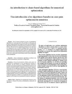
Figure 2.2: A saddle point in IR2 .
∇2 f (x� ) is indefinite, the point x� is neither a local minimum neither a local maximum. Such a point is called a saddle point (see Figure 2.2 for a geometrical illustration). If x� is a stationary point and ∇2 f (x� ) is semi-definite it is not possible to draw any conclusion on the point x� without further knowledge on the function f . Nevertheless, if n = 1 and the function f is infinitely times differentiable it is possible to establish the following necessary and sufficient condition. Proposition 5 Let f : IR → IR and assume f is infinitely times differentiable. The point x� is a local minimum if and only if there exists an even integer r > 1 such that dk f (x� ) =0 dxk for k = 1, 2, . . . , r − 1 and dr f (x� ) > 0. dxr Necessary and sufficient conditions for n > 1 can be only derived if further hypotheses on the function f are added, as shown for example in the following fact. Proposition 6 (Necessary and sufficient condition for convex functions) Let f : IRn → IR and assume ∇f exists and it is continuous. Suppose f is convex, i.e. f (y) − f (x) ≥ ∇f (x)� (y − x)
(2.2)
for all x ∈ IRn and y ∈ IRn . The point x� is a global minimum if and only if ∇f (x� ) = 0.
2.3. GENERAL PROPERTIES OF MINIMIZATION ALGORITHMS
17
Proof. The necessity is a consequence of Theorem 1. For the sufficiency note that, by equation (2.2), if ∇f (x� ) = 0 then f (y) ≥ f (x� ), for all y ∈ IRn .
�
From the above discussion it is clear that to establish the property that x� , satisfying ∇f (x� ) = 0, is a global minimum it is enough to assume that the function f has the following property: for all x and y such that ∇f (x)� (y − x) ≥ 0 one has f (y) ≥ f (x). A function f satisfying the above property is said pseudo-convex. Note that a differentiable convex function is also pseudo-convex, but the opposite is not true. For example, the function x + x3 is pseudo-convex but it is not convex. Finally, if f is strictly convex or strictly pseudo-convex the global minimum (if it exists) is also unique.
2.3
General properties of minimization algorithms
Consider the problem of minimizing the function f : IRn → IR and suppose that ∇f and ∇2 f exist and are continuous. Suppose that such a problem has a solution, and moreover that there exists x0 such that the level set L(f (x0 )) = {x ∈ IRn : f (x) ≤ f (x0 )} is compact. General unconstrained minimization algorithms allow only to determine stationary points of f , i.e. to determine points in the set Ω = {x ∈ IRn : ∇f (x) = 0}. Moreover, for almost all algorithms, it is possible to exclude that the points of Ω yielded by the algorithm are local maxima. Finally, some algorithms yield points of Ω that satisfy also the second order necessary conditions.
2.3.1
General unconstrained minimization algorithm
An algorithm for the solution of the considered minimization problem is a sequence {xk }, obtained starting from an initial point x0 , having some convergence properties in relation with the set Ω. Most of the algorithms that will be studied in this notes can be described in the following general way. 1. Fix a point x0 ∈ IRn and set k = 0.
CHAPTER 2. UNCONSTRAINED OPTIMIZATION
18 2. If xk ∈ Ω STOP.
3. Compute a direction of research dk ∈ IRn . 4. Compute a step αk ∈ IR along dk . 5. Let xk+1 = xk + αk dk . Set k = k + 1 and go back to 2. The existing algorithms differ in the way the direction of research dk is computed and on the criteria used to compute the step αk . However, independently from the particular selection, it is important to study the following issues: • the existence of accumulation points for the sequence {xk }; • the behavior of such accumulation points in relation with the set Ω; • the speed of convergence of the sequence {xk } to the points of Ω.
2.3.2
Existence of accumulation points
To make sure that any subsequence of {xk } has an accumulation point it is necessary to assume that the sequence {xk } remains bounded, i.e. that there exists M > 0 such that �xk � < M for any k. If the level set L(f (x0 )) is compact, the above condition holds if {xk } ∈ L(f (x0 )). This property, in turn, is guaranteed if f (xk+1 ) < f (xk ), for any k such that xk �∈ Ω. The algorithms that satisfy this property are denominated descent methods. For such methods , if L(f (x0 )) is compact and if ∇f is continuous one has • {xk } ∈ L(f (x0 )) and any subsequence of {xk } admits a subsequence converging to a point of L(f (x0 )); • the sequence {f (xk )} has a limit, i.e. there exists f¯ ∈ IR such that lim f (xk ) = f¯;
k→∞
• there always exists an element of Ω in L(f (x0 )). In fact, as f has a minimum in L(f (x0 )), this minimum is also a minimum of f in IRn . Hence, by the assumptions of ∇f , such a minimum must be a point of Ω. Remark. To guarantee the descent property it is necessary that the research directions dk be directions of descent. This is true if ∇f (xk )� dk < 0,
2.3. GENERAL PROPERTIES OF MINIMIZATION ALGORITHMS
19
for all k. Under this condition there exists an interval (0, α� ] such that f (xk + αdk ) < f (xk ), for any α ∈ (0, α� ].
�
Remark. The existence of accumulation points for the sequence {xk } and the convergence of the sequence {f (xk )} do not guarantee that the accumulation points of {xk } are local minima of f or stationary points. To obtain this property it is necessary to impose further � restrictions on the research directions dk and on the steps αk .
2.3.3
Condition of angle
The condition which is in general imposed on the research directions dk is the so-called condition of angle, that can be stated as follows. Condition 1 There exists > 0, independent from k, such that ∇f (xk )� dk ≤ − �∇f (xk )��dk �, for any k. From a geometric point of view the above condition implies that the cosine of the angle between dk and −∇f (xk ) is larger than a certain quantity. This condition is imposed to avoid that, for some k, the research direction is orthogonal to the direction of the gradient. Note moreover that, if the angle condition holds, and if ∇f (xk ) �= 0 then dk is a descent direction. Finally, if ∇f (xk ) �= 0, it is always possible to find a direction dk such that the angle condition holds. For example, the direction dk = −∇f (xk ) is such that the angle condition is satisfied with = 1. Remark. Let {Bk } be a sequence of matrices such that mI ≤ Bk ≤ M I, for some 0 < m < M , and for any k, and consider the directions dk = −Bk ∇f (xk ). Then a simple computation shows that the angle condition holds with = m/M .
�
The angle condition imposes a constraint only on the research directions dk . To make sure that the sequence {xk } converges to a point in Ω it is necessary to impose further conditions on the step αk , as expressed in the following statements. Theorem 4 Let {xk } be the sequence obtained by the algorithm xk+1 = xk + αk dk , for k ≥ 0. Assume that
CHAPTER 2. UNCONSTRAINED OPTIMIZATION
20
(H1) ∇f is continuous and the level set L(f (x0 )) is compact. (H2) There exists > 0 such that ∇f (xk )� dk ≤ − �∇f (xk )��dk �, for any k ≥ 0. (H3) f (xk+1 ) < f (xk ) for any k ≥ 0. (H4) The property
∇f (xk )� dk =0 k→∞ �dk � lim
holds. Then (C1) {xk } ∈ L(f (x0 )) and any subsequence of {xk } has an accumulation point. (C2) {f (xk )} is monotonically decreasing and there exists f¯ such that lim f (xk ) = f¯.
k→∞
(C3) {∇f (xk )} is such that
lim �∇f (xk )� = 0.
k→∞
x) = 0. (C4) Any accumulation point x ¯ of {xk } is such that ∇f (¯ Proof. Conditions (C1) and (C2) are a simple consequence of (H1) and (H3). Note now that (H2) implies |∇f (xk )� dk | , �∇f (xk )� ≤ �dk � for all k. As a result, and by (H4), |∇f (xk )� dk | =0 k→∞ �dk �
lim �∇f (xk )� ≤ lim
k→∞
hence (C3) holds. Finally, let x ¯ be an accumulation point of the sequence {xk }, i.e. there is a subsequence that converges to x ¯. For such a subsequence, and by continuity of f , one has x), lim ∇f (xk ) = ∇f (¯ k→∞
and, by (C3), ∇f (¯ x) = 0, which proves (C4).
�
2.3. GENERAL PROPERTIES OF MINIMIZATION ALGORITHMS
21
Remark. Theorem 4 does not guarantee the convergence of the sequence {xk } to a unique accumulation point. Obviously {xk } has a unique accumulation point if either Ω∩L(f (x0 )) contains only one point or x, y ∈ Ω ∩ L(f (x0 )), with x �= y implies f (x) �= f (y). Finally, if the set Ω ∩ L(f (x0 )) contains a finite number of points, a sufficient condition for the existence of a unique accumulation point is lim �xk+1 − xk � = 0.
k→∞
� Remark. The angle condition can be replaced by the following one. There exists η > 0 and q > 0, both independent from k, such that ∇f (xk )� dk ≤ −η�∇f (xk )�q �dk �. � The result illustrated in Theorem 4 requires the fulfillment of the angle condition or of a similar one, i.e. of a condition involving ∇f . In many algorithms that do not make use of the gradient it may be difficult to check the validity of the angle condition, hence it is necessary to use different conditions on the research directions. For example, it is possible to replace the angle condition with a property of linear independence of the research directions. Theorem 5 Let {xk } be the sequence obtained by the algorithm xk+1 = xk + αk dk , for k ≥ 0. Assume that • ∇2 f is continuous and the level set L(f (x0 )) is compact. • There exist σ > 0, independent from k, and k0 > 0 such that, for any k ≥ k0 the matrix Pk composed of the columns dk+1 dk+n−1 dk , ,..., , �dk � �dk+1 � �dk+n−1 � is such that |detPk | ≥ σ. • limk→∞ �xk+1 − xk � = 0. • f (xk+1 ) < f (xk ) for any k ≥ 0. • The property
∇f (xk )� dk =0 k→∞ �dk � lim
holds.
CHAPTER 2. UNCONSTRAINED OPTIMIZATION
22 Then
• {xk } ∈ L(f (x0 )) and any subsequence of {xk } has an accumulation point. • {f (xk )} is monotonically decreasing and there exists f¯ such that lim f (xk ) = f¯.
k→∞
x) = 0. • Any accumulation point x ¯ of {xk } is such that ∇f (¯ Moreover, if the set Ω ∩ L(f (x0 )) is composed of a finite number of points, the sequence {xk } has a unique accumulation point.
2.3.4
Speed of convergence
Together with the property of convergence of the sequence {xk } it is important to study also the speed of convergence. To study such a notion it is convenient to assume that {xk } converges to a point x� . If there exists a finite k such that xk = x� then we say that the sequence {xk } has finite convergence. Note that if {xk } is generated by an algorithm, there is a stopping condition that has to be satisfied at step k. If xk �= x� for any finite k, it is possible (and convenient) to study the asymptotic properties of {xk }. One criterion to estimate the speed of convergence is based on the behavior of the error Ek = �xk − x� �, and in particular on the relation between Ek+1 and Ek . We say that {xk } has speed of convergence of order p if �
lim
k→∞
Ek+1 Ekp
= Cp
with p ≥ 1 and 0 < Cp < ∞. Note that if {xk } has speed of convergence of order p then �
lim
k→∞
if 1 ≤ q < p, and
�
lim
k→∞
Ek+1 Ekq
Ek+1 Ekq
= 0,
= ∞,
if q > p. Moreover, from the definition of speed of convergence, it is easy to see that if {xk } has speed of convergence of order p then, for any > 0 there exists k0 such that Ek+1 ≤ (Cp + )Ekp , for any k > k0 . In the cases p = 1 or p = 2 the following terminology is often used. If p = 1 and 0 < C1 ≤ 1 the speed of convergence is linear; if p = 1 and C1 > 1 the speed of convergence is sublinear; if
Ek+1 =0 lim k→∞ Ek
2.4. LINE SEARCH
23
the speed of convergence is superlinear, and finally if p = 2 the speed of convergence is quadratic. Of special interest in optimization is the case of superlinear convergence, as this is the kind of convergence that can be established for the efficient minimization algorithms. Note that if xk has superlinear convergence to x� then �xk+1 − xk � = 1. k→∞ �xk − x� � lim
Remark. In some cases it is not possible to establish the existence of the limit �
lim
k→∞
Ek+1 Ekq
.
In these cases an estimate of the speed of convergence is given by �
Ek+1 Qp = lim sup Ekq k→∞
. �
2.4
Line search
A line search is a method to compute the step αk along a given direction dk . The choice of αk affects both the convergence and the speed of convergence of the algorithm. In any line search one considers the function of one variable φ : IR → IR defined as φ(α) = f (xk + αdk ) − f (xk ). The derivative of φ(α) with respect to α is given by ˙ φ(α) = ∇f (xk + αdk )� dk provided that ∇f is continuous. Note that ∇f (xk + αdk )� dk describes the slope of the tangent to the function φ(α), and in particular ˙ φ(0) = ∇f (xk )� dk coincides with the directional derivative of f at xk along dk . From the general convergence results described, we conclude that the line search has to enforce the following conditions f (xk+1 ) < f (xk ) ∇f (xk )� dk =0 k→∞ �dk � lim
CHAPTER 2. UNCONSTRAINED OPTIMIZATION
24
and, whenever possible, also the condition lim �xk+1 − xk � = 0.
k→∞
To begin with, we assume that the directions dk are such that ∇f (xk )� dk < 0 for all k, i.e. dk is a descent direction, and that it is possible to compute, for any fixed x, both f and ∇f . Finally, we assume that the level set L(f (x0 )) is compact.
2.4.1
Exact line search
The exact line search consists in finding αk such that φ(αk ) = f (xk + αk dk ) − f (xk ) ≤ f (xk + αdk ) − f (xk ) = φ(α) for any α ≥ 0. Note that, as dk is a descent direction and the set {α ∈ IR+ : φ(α) ≤ φ(0)} is compact, because of compactness of L(f (x0 )), there exists an αk that minimizes φ(α). Moreover, for such αk one has ˙ k ) = ∇f (xk + αk dk )� dk = 0, φ(α i.e. if αk minimizes φ(α) the gradient of f at xk + αk dk is orthogonal to the direction dk . From a geometrical point of view, if αk minimizes φ(α) then the level surface of f through the point xk + αk dk is tangent to the direction dk at such a point. (If there are several points of tangency, αk is the one for which f has the smallest value). The search of αk that minimizes φ(α) is very expensive, especially if f is not convex. Moreover, in general, the whole minimization algorithm does not gain any special advantage from the knowledge of such optimal αk . It is therefore more convenient to use approximate methods, i.e. methods which are computationally simple and which guarantee particular convergence properties. Such methods are aimed at finding an interval of acceptable values for αk subject to the following two conditions • αk has to guarantee a sufficient reduction of f ; • αk has to be sufficiently distant from 0, i.e. xk + αk dk has to be sufficiently away from xk .
2.4.2
Armijo method
Armijo method was the first non-exact linear search method. Let a > 0, σ ∈ (0, 1) and γ ∈ (0, 1/2) be given and define the set of points A = {α ∈ R : α = aσ j , j = 0, 1, . . .}.
2.4. LINE SEARCH
25
φ(0)
σa
α
a φ(α)
.
γ φ(0)α
.
φ(0)α Figure 2.3: Geometrical interpretation of Armijo method.
Armijo method consists in finding the largest α ∈ A such that ˙ φ(α) = f (xk + αdk ) − f (xk ) ≤ γα∇f (xk )� dk = γαφ(0). Armijo method can be implemented using the following (conceptual) algorithm. Step 1. Set α = a. Step 2. If
f (xk + αdk ) − f (xk ) ≤ γα∇f (xk )� dk
set αk = α and STOP. Else go to Step 3. Step 3. Set α = σα, and go to Step 2. From a geometric point of view (see Figure 2.3) the condition in Step 2 requires that αk is such that φ(αk ) is below the straight line passing through the point (0, φ(0)) and with ˙ ˙ slope γ φ(0). Note that, as γ ∈ (0, 1/2) and φ(0) < 0, such a straight line has a slope smaller than the slope of the tangent at the curve φ(α) at the point (0, φ(0)). For Armijo method it is possible to prove the following convergence result. Theorem 6 Let f : IRn → IR and assume ∇f is continuous and L(f (x0 )) is compact. Assume ∇f (xk )� dk < 0 for all k and there exist C1 > 0 and C2 > 0 such that C1 ≥ �dk � ≥ C2 �∇f (xk )�q , for some q > 0 and for all k. Then Armijo method yields in a finite number of iterations a value of αk > 0 satisfying the condition in Step 2. Moreover, the sequence obtained setting xk+1 = xk + αk dk is such that f (xk+1 ) < f (xk ),
CHAPTER 2. UNCONSTRAINED OPTIMIZATION
26 for all k, and
∇f (xk )� dk = 0. k→∞ �dk � lim
Proof. We only prove that the method cannot loop indefinitely between Step 2 and Step 3. In fact, if this is the case, then the condition in Step 2 will never be satisfied, hence f (xk + aσ j dk ) − f (xk ) > γ∇f (xk )� dk . aσ j Note now that σ j → 0 as j → ∞, and the above inequality for j → ∞ is ∇f (xk )� dk > γ∇f (xk )� dk , which is not possible since γ ∈ (0, 1/2) and ∇f (xk )� dk �= 0.
�
Remark. It is interesting to observe that in Theorem 6 it is not necessary to assume that xk+1 = xk + αk dk . It is enough that xk+1 is such that f (xk+1 ) ≤ f (xk + αk dk ), where αk is generated using Armijo method. This implies that all acceptable values of α are those such that f (xk + αdk ) ≤ f (xk + αk dk ). As a result, Theorem 6 can be used to prove also the convergence of an algorithm based on the exact line search. �
2.4.3
Goldstein conditions
The main disadvantage of Armijo method is in the fact that, to find αk , all points in the set A, starting from the point α = a, have to be tested till the condition in Step 2 is fulfilled. There are variations of the method that do not suffer from this disadvantage. A criterion similar to Armijo’s, but that allows to find an acceptable αk in one step, is based on the so-called Goldstein conditions. Goldstein conditions state that given γ1 ∈ (0, 1) and γ2 ∈ (0, 1) such that γ1 < γ2 , αk is any positive number such that f (xk + αk dk ) − f (xk ) ≤ αk γ1 ∇f (xk )� dk i.e. there is a sufficient reduction in f , and f (xk + αk dk ) − f (xk ) ≥ αk γ2 ∇f (xk )� dk i.e. there is a sufficient distance between xk and xk+1 . From a geometric point of view (see Figure 2.4) this is equivalent to select αk as any point such that the corresponding value of f is included between two straight lines, of slope
2.4. LINE SEARCH
27
α
α
φ(0)
α φ(α)
.
γ1φ(0)α
.
φ(0)α
.
γ2φ(0)α
Figure 2.4: Geometrical interpretation of Goldstein method.
γ1 ∇f (xk )� dk and γ2 ∇f (xk )� dk , respectively, and passing through the point (0, φ(0)). As 0 < γ1 < γ2 < 1 it is obvious that there exists always an interval I = [α, α] such that Goldstein conditions hold for any α ∈ I. Note that, a result similar to Theorem 6, can be also established if the sequence {xk } is generated using Goldstein conditions. The main disadvantage of Armijo and Goldstein methods is in the fact that none of them impose conditions on the derivative of the function φ(α) in the point αk , or what is the same on the value of ∇f (xk+1 )� dk . Such extra conditions are sometimes useful in establishing convergence results for particular algorithms. However, for simplicity, we omit the discussion of these more general conditions (known as Wolfe conditions).
2.4.4
Line search without derivatives
It is possible to construct methods similar to Armijo’s or Goldstein’s also in the case that no information on the derivatives of the function f is available. Suppose, for simplicity, that �dk � = 1, for all k, and that the sequence {xk } is generated by xk+1 = xk + αk dk . If ∇f is not available it is not possible to decide a priori if the direction dk is a descent direction, hence it is necessary to consider also negative values of α. We now describe the simplest line search method that can be constructed with the considered hypothesis. This method is a modification of Armijo method and it is known as parabolic search. Given λ0 > 0, σ ∈ (0, 1/2), γ > 0 and ρ ∈ (0, 1). Compute αk and λk such that one of the following conditions hold. Condition (i)
CHAPTER 2. UNCONSTRAINED OPTIMIZATION
28 • λk = λk−1 ;
• αk is the largest value in the set A = {α ∈ IR : α = ±σ j , j = 0, 1, . . .} such that f (xk + αk dk ) ≤ f (xk ) − γα2k , or, equivalently, φ(αk ) ≤ −γα2k . Condition (ii) • αk = 0, λk ≤ ρλk−1 ; • min (f (xk + λk dk ), f (xk − λk dk )) ≥ f (xk ) − γλ2k . At each step it is necessary to satisfy either Condition (i) or Condition (ii). Note that this is always possible for any dk �= 0. Condition (i) requires that αk is the largest number in the set A such that f (xk + αk dk ) is below the parabola f (xk ) − γα2 . If the function φ(α) has a stationary point for α = 0 then there may be no α ∈ A such that Condition (i) holds. However, in this case it is possible to find λk such that Condition (ii) holds. If Condition (ii) holds then αk = 0, i.e. the point xk remains unchanged and the algorithms continues with a new direction dk+1 �= dk . For the parabolic search algorithm it is possible to prove the following convergence result. Theorem 7 Let f : IRn → IR and assume ∇f is continuous and L(f (x0 )) is compact. If αk is selected following the conditions of the parabolic search and if xk+1 = xk + αk dk , with �dk � = 1 then the sequence {xk } is such that f (xk+1 ) ≤ f (xk ) for all k, lim ∇f (xk )� dk = 0
k→∞
and lim �xk+1 − xk � = 0.
k→∞
Proof. (Sketch) Note that Condition (i) implies f (xk+1 ) < f (xk ), whereas Condition (ii) ¯ then αk = 0 implies f (xk+1 ) = f (xk ). Note now that if Condition (ii) holds for all k ≥ k, ¯ for all k ≥ k, i.e. �xk+1 − xk � = 0. Moreover, as λk is reduced at each step, necessarily � ∇f (xk¯ )� d¯ = 0, where d¯ is a limit of the sequence {dk }.
2.5. THE GRADIENT METHOD
2.4.5
29
Implementation of a line search algorithm
On the basis of the conditions described so far it is possible to construct algorithms that yield αk in a finite number of steps. One such an algorithm can be described as follows. (For simplicity we assume that ∇f is known.) • Initial data. xk , f (xk ), ∇f (xk ), α and α. • Initial guess for α. A possibility is to select α as the point in which a parabola ˙ through (0, φ(0)) with derivative φ(0) for α = 0 takes a pre-specified minimum value f� . Initially, i.e. for k = 0, f� has to be selected by the designer. For k > 0 it is possible to select f� such that f (xk ) − f� = f (xk−1 ) − f (xk ). The resulting α is α� = −2
f (xk ) − f� . ∇f (xk )� dk
In some algorithms it is convenient to select α ≤ 1, hence the initial guess for α will be min (1, α� ) . • Computation of αk . A value for αk is computed using a line search method. If αk ≤ α the direction dk may not be a descent direction. If αk ≥ α the level set L(f (xk )) may not be compact. If αk �∈ [α, α] the line search fails, and it is necessary to select a new research direction dk . Otherwise the line search terminates and xk+1 = xk + αk dk .
2.5
The gradient method
The gradient method consists in selecting, as research direction, the direction of the antigradient at xk , i.e. dk = −∇f (xk ), for all k. This selection is justified noting that the direction7 −
∇f (xk ) �∇f (xk )�E
is the direction that minimizes the directional derivative, among all direction with unitary Euclidean norm. In fact, by Schwartz inequality, one has |∇f (xk )� d| ≤ �d�E �∇f (xk )�E , and the equality sign holds if and only if d = λ∇f (xk ), with λ ∈ IR. As a consequence, the problem min ∇f (xk )� d �d�E =1
7
We denote with �v�E the Euclidean norm of the vector v, i.e. �v�E =
√
v � v.
CHAPTER 2. UNCONSTRAINED OPTIMIZATION
30
∇f (xk ) has the solution d� = − �∇f (xk )�E . For this reason, the gradient method is sometimes called the method of the steepest descent. Note however that the (local) optimality of the direction −∇f (xk ) depends upon the selection of the norm, and that with a proper selection of the norm, any descent direction can be regarded as the steepest descent. The real interest in the direction −∇f (xk ) rests on the fact that, if ∇f is continuous, then the former is a continuous descent direction, which is zero only if the gradient is zero, i.e. at a stationary point. The gradient algorithm can be schematized has follows.
Step 0. Given x0 ∈ IRn . Step 1. Set k = 0. Step 2. Compute ∇f (xk ). If ∇f (xk ) = 0 STOP. Else set dk = −∇f (xk ). Step 3. Compute a step αk along the direction dk with any line search method such that f (xk + αk dk ) ≤ f (xk ) and
∇f (xk )� dk = 0. k→∞ �dk � lim
Step 4. Set xk+1 = xk + αk dk , k = k + 1. Go to Step 2. By the general results established in Theorem 4, we have the following fact regarding the convergence properties of the gradient method. Theorem 8 Consider f : IRn → IR. Assume ∇f is continuous and the level set L(f (x0 )) is compact. Then any accumulation point of the sequence {xk } generated by the gradient algorithm is a stationary point of f .
3
2.5
2
1.5
1
0.5
0
1
2
3
4
5
6
7
Figure 2.5: The function
8
9
�
ξ
10
ξ−1 . ξ+1
2.6. NEWTON’S METHOD
31
To estimate the speed of convergence of the method we can consider the behavior of the method in the minimization of a quadratic function, i.e. in the case 1 f (x) = x� Qx + c� x + d, 2 with Q = Q� > 0. In such a case it is possible to obtain the following estimate
�xk+1 − x� � ≤
�
λM λM λ −1 � m �xk − x� �, λM λm + 1 λm
where λM ≥ λm > 0 are the maximum and minimum eigenvalue of Q, respectively. Note that the above estimate is exact for some initial points x0 . As a result, if λM �= λm the gradient algorithm has linear convergence, however, if λM /λm is large the convergence can be very slow (see Figure 2.5). Finally, if λM /λm = 1 the gradient algorithm converges in one step. From a geometric point of view the ratio λM /λm expresses the ratio between the lengths of the maximum and the minimum axes of the ellipsoids, that constitute the level surfaces of f . If this ratio is big there are points from which the gradient algorithm converges very slowly, see e.g. Figure 2.6.
. . . . Figure 2.6: Behavior of the gradient algorithm.
In the non-quadratic case, the performance of the gradient method are unacceptable, especially if the level surfaces of f have high curvature.
2.6
Newton’s method
Newton’s method, with all its variations, is the most important method in unconstrained optimization. Let f : IRn → IR be a given function and assume that ∇2 f is continuous. Newton’s method for the minimization of f can be derived assuming that, given xk , the point xk+1 is obtained minimizing a quadratic approximation of f . As f is two times differentiable, it is possible to write 1 f (xk + s) = f (xk ) + ∇f (xk )� s + s� ∇2 f (xk )s + β(xk , s), 2 in which lim
�s�→0
β(xk , s) = 0. �s�2
CHAPTER 2. UNCONSTRAINED OPTIMIZATION
32
For �s� sufficiently small, it is possible to approximate f (xk + s) with its quadratic approximation 1 q(s) = f (xk ) + ∇f (xk )� s + s� ∇2 f (xk )s. 2 If ∇2 f (xk ) > 0, the value of s minimizing q(s) can be obtained setting to zero the gradient of q(s), i.e. ∇q(s) = ∇f (xk ) + ∇2 f (xk )s = 0, yielding
�
�−1
s = − ∇2 f (xk )
∇f (xk ).
The point xk+1 is thus given by �
�−1
xk+1 = xk − ∇2 f (xk )
∇f (xk ).
Finally, Newton’s method can be described by the simple scheme. Step 0. Given x0 ∈ IRn . Step 1. Set k = 0. Step 2. Compute
�
�−1
s = − ∇2 f (xk )
∇f (xk ).
Step 3. Set xk+1 = xk + s, k = k + 1. Go to Step 2. Remark. An equivalent way to introduce Newton’s method for unconstrained optimization is to regard the method as an algorithm for the solution of the system of n non-linear equations in n unknowns given by ∇f (x) = 0. For, consider, in general, a system of n equations in n unknown F (x) = 0, with x ∈ IRn and F : IRn → IRn . If the Jacobian matrix of F exists and is continuous, then one can write ∂F (x)s + γ(x, s), F (x + s) = F (x) + ∂x with γ(x, s) = 0. lim �s�→0 �s� Hence, given a point xk we can determine xk+1 = xk + s setting s such that F (xk ) +
∂F (xk )s = 0. ∂x
2.6. NEWTON’S METHOD If
∂F ∂x (xk )
33
is invertible we have �
s=−
�−1
∂F (xk ) ∂x
F (xk ),
hence Newton’s method for the solution of the system of equation F (x) = 0 is �
xk+1
�−1
∂F (xk ) = xk − ∂x
F (xk ),
(2.3)
with k = 0, 1, . . .. Note that, if F (x) = ∇f , then the above iteration coincides with Newton’s method for the minimization of f . � To study the convergence properties of Newton’s method we can consider the algorithm for the solution of a set of non-linear equations, summarized in equation (2.3). The following local convergence result, providing also an estimate of the speed of convergence, can be proved. Theorem 9 Let F : IRn → IRn and assume that F is continuously differentiable in an open set D ⊂ IRn . Suppose moreover that • there exists x� ∈ D such that F (x� ) = 0; • the Jacobian matrix
∂F ∂x (x� )
is non-singular;
• there exists L > 0 such that8
� � � ∂F � ∂F � � � ∂x (z) − ∂x (y)� ≤ L�z − y�,
for all z ∈ D and y ∈ D. Then there exists and open set B ⊂ D such that for any x0 ∈ B the sequence {xk } generated by equation (2.3) remains in B and converges to x� with quadratic speed of convergence. The result in Theorem 9 can be easily recast as a result for the convergence of Newton’s method for unconstrained optimization. For, it is enough to note that all hypotheses 2 on F and ∂F ∂x translate into hypotheses on ∇f and ∇ f . Note however that the result is only local and does not allow to distinguish between local minima and local maxima. To construct an algorithm for which the sequence {xk } does not converge to maxima, and for which global convergence, i.e. convergence from points outside the set B, holds, it is possible to �modify Newton’s method considering a line search along the direction � −1 ∇f (xk ). As a result, the modified Newton’s algorithm dk = − ∇2 f (xk ) �
�−1
xk+1 = xk − αk ∇2 f (xk ) 8
This is equivalent to say that
∂F ∂x
∇f (xk ),
(x) is Lipschitz continuous in D.
(2.4)
CHAPTER 2. UNCONSTRAINED OPTIMIZATION
34
in which αk is computed using any line search algorithm, is obtained. If ∇2 f is uniformly �positive definite, and this implies that the function f is convex, the direction �−1 ∇f (xk ) is a descent direction satisfying the condition of angle. Hence, dk = − ∇2 f (xk ) by Theorem 4, we can conclude the (global) convergence of the algorithm (2.4). Moreover, it is possible to prove that, for k sufficiently large, the step αk = 1 satisfies the conditions of Armijo method, hence the sequence {xk } has quadratic speed of convergence. Remark. If the function to be minimized is quadratic, i.e. 1 f (x) = x� Qx + c� x + d, 2 and if Q > 0, Newton’s method yields the (global) minimum of f in one step.
�
In general, i.e. if ∇2 f (x) is not positive definite for all x, Newton’s method may be in� �−1 applicable because either ∇2 f (xk ) is not invertible, or dk = − ∇2 f (xk ) ∇f (xk ) is not a descent direction. In these cases it is necessary to further modify Newton’s method. Diverse criteria have been proposed, most of which rely on the substitution of the matrix ∇2 f (xk ) with a matrix Mk > 0 which is close in some sense to ∇2 f (xk ). A simpler modification can be obtained using the direction dk = −∇f (xk ) whenever the direction � �−1 ∇f (xk ) is not a descent direction. This modification yields the foldk = − ∇2 f (xk ) lowing algorithm. Step 0. Given x0 ∈ IRn and > 0. Step 1. Set k = 0. Step 2. Compute ∇f (xk ). If ∇f (xk ) = 0 STOP. Else compute ∇2 f (xk ). If ∇2 f (xk ) is singular set dk = −∇f (xk ) and go to Step 6. Step 3. Compute Newton direction s solving the (linear) system ∇2 f (xk )s = −∇f (xk ). Step 4. If
|∇f (xk )� s| < �∇f (xk )��s�
set dk = −∇f (xk ) and go to Step 6. Step 5. If set dk = s; if
∇f (xk )� s < 0 ∇f (xk )� s > 0
set dk = −s. Step 6. Make a line search along dk assuming as initial estimate α = 1. Compute xk+1 = xk + αk dk , set k = k + 1 and go to Step 2.
2.6. NEWTON’S METHOD
35
The above algorithm is such that the direction dk satisfies the condition of angle, i.e. ∇f (xk )� dk ≤ − �∇f (xk )��dk �, for all k. Hence, the convergence is guaranteed by the general result in Theorem 4. Moreover, if is sufficiently small, if the hypotheses of Theorem 9 hold, and if the line search is performed with Armijo method and with the initial guess α = 1, then the above algorithm has quadratic speed of convergence. Finally, note that it is possible to modify Newton’s method, whenever it is not applicable, without making use of the direction of the anti-gradient. We now briefly discuss two such modifications.
2.6.1
Method of the trust region
A possible approach to modify Newton’s method to yield global convergence is to set the direction dk and the step αk in such a way to minimize the quadratic approximation of f on a sphere centered at xk and of radius ak . Such a sphere is called trust region. This name refers to the fact that, in a small region around xk we are confident (we trust) that the quadratic approximation of f is a good approximation. The method of the trust region consists in selecting xk+1 = xk +sk , where sk is the solution of the problem (2.5) min q(s), �s�≤ak
with
1 q(s) = f (xk ) + ∇f (xk )� s + s� ∇2 f (xk )s, 2
and ak > 0 the estimate at step k of the trust region. As the above (constrained) optimization problem has always a solution, the direction sk is always defined. The computation of the estimate ak is done, iteratively, in such a way to enforce the condition f (xk+1 ) < f (xk ) and to make sure that f (xk + sk ) ≈ q(sk ), i.e. that the change of f and the estimated change of f are close. Using these simple ingredients it is possible to construct the following algorithm. Step 0. Given x0 ∈ IRn and a0 > 0. Step 1. Set k = 0. Step 2. Compute ∇f (xk ). If ∇f (xk ) = 0 STOP. Else go to Step 3. Step 3. Compute sk solving problem (2.5). Step 4. Compute9 ρk = 9
If f is quadratic then ρk = 1 for all k.
f (xk + sk ) − f (xk ) . q(sk ) − f (xk )
(2.6)
CHAPTER 2. UNCONSTRAINED OPTIMIZATION
36
Step 5. If ρk < 1/4 set ak+1 = �sk �/4. If ρk > 3/4 and �sk � = ak set ak+1 = 2ak . Else set ak+1 = ak . Step 6. If ρk ≤ 0 set xk+1 = xk . Else set xk+1 = xk + sk . Step 7. Set k = k + 1 and go to Step 2. Remark. Equation (2.6) expresses the ratio between the actual change of f and the estimated change of f . � It is possible to prove that, if L(f (x0 )) is compact and ∇2 f is continuous, any accumulation point resulting from the above algorithm is a stationary point of f , in which the second order necessary conditions hold. The update of ak is devised to enlarge or shrink the region of confidence on the basis of the number ρk . It is possible to show that if {xk } converges to a local minimum in which ∇2 f is positive definite, then ρk converges to one and the direction sk coincides, for k sufficiently large, with the Newton direction. As a result, the method has quadratic speed of convergence. In practice, the solution of the problem (2.5) cannot be obtained analytically, hence approximate problems have to be solved. For, consider sk as the solution of the equation �
�
∇2 f (xk ) + νk I sk = −∇f (xk ),
(2.7)
in which νk > 0 has to be determined with proper considerations. Under certain hypotheses, the sk determined solving equation (2.7) coincides with the sk computed using the method of the trust region. Remark. A potential disadvantage of the method of the trust region is to reduce the step � along Newton direction even if the selection αk = 1 would be feasible.
2.6.2
Non-monotonic line search
Experimental evidence shows that Newton’s method gives the best result if the step αk = 1 is used. Therefore, the use of αk < 1 along Newton direction, resulting e.g. from the application of Armijo method, results in a degradation of the performance of the algorithm. To avoid this phenomenon it has been suggested to relax the condition f (xk+1 ) < f (xk ) imposed on Newton algorithm, thus allowing the function f to increase for a certain number of steps. For example, it is possible to substitute the reduction condition of Armijo method with the condition f (xk + αk dk ) ≤ max [f (xk−j )] + γαk ∇f (xk )� dk 0≤j≤M
for all k ≥ M , where M > 0 is a fixed integer independent from k.
2.7. CONJUGATE DIRECTIONS METHODS
37
Gradient method
Newton’s method
Information required at each step
f and ∇f
f , ∇f and ∇2 f
Computation to find the research direction
∇f (xk )
∇f (xk ), ∇2 f (xk ), −[∇2 f (xk )]−1 ∇f (xk )
Convergence Behavior for quadratic functions Speed of convergence
Global if L(f (x0 )) compact and ∇f continuous Asymptotic convergence
Convergence in one step
Linear for quadratic functions
Quadratic (under proper hypotheses)
Local, but may be rendered global
Table 2.1: Comparison between the gradient method and Newton’s method.
2.6.3
Comparison between Newton’s method and the gradient method
The gradient method and Newton’s method can be compared from different point of views, as described in Table 2.1. From the table, it is obvious that Newton’s method has better convergence properties but it is computationally more expensive. There exist methods which preserve some of the advantages of Newton’s method, namely speed of convergence faster than the speed of the gradient method and finite convergence for quadratic functions, without requiring the knowledge of ∇2 f . Such methods are • the conjugate directions methods; • quasi-Newton methods.
2.7
Conjugate directions methods
Conjugate directions methods have been motivated by the need of improving the convergence speed of the gradient method, without requiring the computation of ∇2 f , as required in Newton’s method. A basic characteristic of conjugate directions methods is to find the minimum of a quadratic function in a finite number of steps. These methods have been introduced for the solution of systems of linear equations and have later been extended to the solution of unconstrained optimization problems for non-quadratic functions.
CHAPTER 2. UNCONSTRAINED OPTIMIZATION
38
Definition 5 Given a matrix Q = Q� , the vectors d1 and d2 are said to be Q-conjugate if d�1 Qd2 = 0. Remark. If Q = I then two vectors are Q-conjugate if they are orthogonal.
�
Theorem 10 Let Q ∈ IRn×n and Q = Q� > 0. Let di ∈ IRn , for i = 0, · · · , k, be non-zero vectors. If di are mutually Q-conjugate, i.e. d�i Qdj = 0, for all i �= j, then the vectors di are linearly independent. Proof. Suppose there exists constants αi , with αi �= 0 for some i, such that α0 d0 + · · · αk dk = 0. Then, left multiplying with Q and d�j yields αj d�j Qdj = 0, which implies, as Q > 0, αj = 0. Repeating the same considerations for all j ∈ [0, k] yields the claim. � Consider now a quadratic function 1 f (x) = x� Qx + c� x + d, 2 with x ∈ IRn and Q = Q� > 0. The (global) minimum of f is given by x� = −Q−1 c, and this can be computed using the procedure given in the next statement. Theorem 11 Let Q = Q� > 0 and let d0 , d1 , · · ·, dn−1 be n non-zero vectors mutually Q-conjugate. Consider the algorithm xk+1 = xk + αk dk with αk = −
∇f (xk )� dk (x� Q + c� )dk =− k � . � dk Qdk dk Qdk
Then, for any x0 , the sequence {xk } converges, in at most n steps, to x� = −Q−1 c, i.e. it converges to the minimum of the quadratic function f .
2.7. CONJUGATE DIRECTIONS METHODS
39
Remark. Note that αk is selected at each step to minimize the function f (xk + αdk ) with respect to α, i.e. at each step an exact line search in the direction dk is performed. � In the above statement we have assumed that the directions dk have been preliminarily assigned. However, it is possible to construct a procedure in which the directions are computed iteratively. For, consider the quadratic function f (x) = 12 x� Qx + c� x + d, with Q > 0, and the following algorithm, known as conjugate gradient method. Step 0. Given x0 ∈ IRn and the direction d0 = −∇f (x0 ) = −(Qx0 + c). Step 1. Set k = 0. Step 2. Let xk+1 = xk + αk dk with αk = −
∇f (xk )� dk (x�k Q + c� )dk − . d�k Qdk d�k Qdk
Step 3. Compute dk+1 as follows dk+1 = −∇f (xk+1 ) + βk dk , with βk =
∇f (xk+1 )� Qdk . d�k Qdk
Step 4. Set k = k + 1 and go to Step 2. Remark. As already observed, αk is selected to minimize the function f (xk + αdk ). Moreover, this selection of αk is also such that ∇f (xk+1 )� dk = 0.
(2.8)
In fact, Qxk+1 = Qxk + αk Qdk hence ∇f (xk+1 ) = ∇f (xk ) + αk Qdk .
(2.9)
Left multiplying with d�k yields d�k ∇f (xk+1 ) = d�k ∇f (xk ) + d�k Qdk αk = d�k ∇f (xk ) − d�k Qdk
∇f (xk )� dk = 0. d�k Qdk �
CHAPTER 2. UNCONSTRAINED OPTIMIZATION
40
Remark. βk is such that dk+1 is Q-conjugate with respect to dk . In fact, �
d�k Qdk+1
∇f (xk+1 )� Qdk = d�k Q −∇f (xk+1 ) + dk d�k Qdk
= d�k Q (−∇f (xk+1 ) + ∇f (xk+1 )) = 0.
Moreover, this selection of βk yields also ∇f (xk )� dk = −∇f (xk )� ∇f (xk ).
(2.10) �
For the conjugate gradient method it is possible to prove the following fact. Theorem 12 The conjugate gradient method yields the minimum of the quadratic function 1 f (x) = x� Qx + c� x + d, 2 � with Q = Q > 0, in at most n iterations, i.e. there exists m ≤ n − 1 such that ∇f (xm+1 ) = 0. Moreover
∇f (xj )� ∇f (xi ) = 0
(2.11)
d�j Qdi = 0,
(2.12)
and for all [0, m + 1] � i �= j ∈ [0, m + 1].
Proof. To prove the (finite) convergence of the sequence {xk } it is enough to show that the directions dk are Q-conjugate, i.e. that equation (2.12) holds. In fact, if equation (2.12) holds the claim is a consequence of Theorem 11. � The conjugate gradient algorithm, in the form described above, cannot be used for the minimization of non-quadratic functions, as it requires the knowledge of the matrix Q, which is the Hessian of the function f . Note that the matrix Q appears at two levels in the algorithm: in the computation of the scalar βk required to compute the new direction of research, and in the computation of the step αk . It is therefore necessary to modify the algorithm to avoid the computation of ∇2 f , but at the same time it is reasonable to make sure that the modified algorithm coincides with the above one in the quadratic case.
2.7.1
Modification of βk
To begin with note that, by equation (2.9), βk can be written as ∇f (xk+1 ) − ∇f (xk ) ∇f (xk+1 )� [∇f (xk+1 ) − ∇f (xk )] αk , = d�k [∇f (xk+1 ) − ∇f (xk )] � ∇f (xk+1 ) − ∇f (xk ) dk αk
∇f (xk+1 )� βk =
2.7. CONJUGATE DIRECTIONS METHODS
41
and, by equation (2.8), βk = −
∇f (xk+1 )� [∇f (xk+1 ) − ∇f (xk )] . d�k ∇f (xk )
(2.13)
Using equation (2.13), it is possible to construct several expressions for βk , all equivalent in the quadratic case, but yielding different algorithms in the general (non-quadratic) case. A first possibility is to consider equations (2.10) and (2.11) and to define βk =
∇f (xk+1 )� ∇f (xk+1 ) �∇f (xk+1 )�2 , = ∇f (xk )� ∇f (xk ) �∇f (xk )�2
(2.14)
which is known as Fletcher-Reeves formula. A second possibility is to write the denominator as in equation (2.14) and the numerator as in equation (2.13), yielding βk =
∇f (xk+1 )� [∇f (xk+1 ) − ∇f (xk )] , �∇f (xk )�2
(2.15)
which is known as Polak-Ribiere formula. Finally, it is possible to have the denominator as in (2.13) and the numerator as in (2.14), i.e. βk = −
2.7.2
�∇f (xk+1 )�2 . d�k ∇f (xk )
(2.16)
Modification of αk
As already observed, in the quadratic version of the conjugate gradient method also the step αk depends upon Q. However, instead of using the αk given in Step 2 of the algorithm, it is possible to use a line search along the direction αk . In this way, an algorithm for non-quadratic functions can be constructed. Note that αk , in the algorithm for quadratic functions, is also such that dk ∇f (xk+1 ) = 0. Therefore, in the line search, it is reasonable to select αk such that, not only f (xk+1 ) < f (xk ), but also dk is approximately orthogonal to ∇f (xk+1 ). Remark. The condition of approximate orthogonality between dk and ∇f (xk+1 ) cannot be enforced using Armijo method or Goldstein conditions. However, there are more sophisticated line search algorithms, known as Wolfe conditions, which allow to enforce the above constraint. �
2.7.3
Polak-Ribiere algorithm
As a result of the modifications discussed in the last sections, it is possible to construct an algorithm for the minimization of general functions. For example, using equation (2.15) we obtain the following algorithm, due to Polak-Ribiere, which has proved to be one of the most efficient among the class of conjugate directions methods.
CHAPTER 2. UNCONSTRAINED OPTIMIZATION
42 Step 0. Given x0 ∈ IRn . Step 1. Set k = 0.
Step 2. Compute ∇f (xk ). If ∇f (xk ) = 0 STOP. Else let ⎧ −∇f (x0 ), ⎪ ⎪ ⎨
dk =
if k = 0
∇f (xk )� [∇f (xk ) − ∇f (xk−1 )] ⎪ ⎪ dk−1 , ⎩ −∇f (xk ) + 2 �∇f (xk−1 )�
if k ≥ 1.
Step 3. Compute αk performing a line search along dk . Step 4. Set xk+1 = xk + αk dk , k = k + 1 and go to Step 2. Remark. The line search has to be sufficiently accurate, to make sure that all directions generated by the algorithm are descent directions. A suitable line search algorithm is the so-called Wolfe method, which is a modification of Goldstein method. � Remark. To guarantee global convergence of a subsequence it is possible to use, every n steps, the direction −∇f . In this case, it is said that the algorithm uses a restart procedure. For the algorithm with restart it is possible to have quadratic speed of convergence in n steps, i.e �xk+n − x� � ≤ γ�xk − x� �2 , for some γ > 0.
�
Remark. It is possible to modify Polak-Ribiere algorithm to make sure that at each step the angle condition holds. In this case, whenever the direction dk does not satisfy the angle condition, it is sufficient to use the direction −∇f . Note that, enforcing the angle condition, yields a globally convergent algorithm. � Remark. Even if the use of the direction −∇f every n steps, or whenever the angle condition is not satisfied, allows to prove global convergence of Polak-Ribiere algorithm, it has been observed in numerical experiments that such modified algorithms do not perform as well as the original one. �
2.8
Quasi-Newton methods
Conjugate gradient methods have proved to be more efficient than the gradient method. However, in general, it is not possible to guarantee superlinear convergence. The main advantage of conjugate gradient methods is in the fact that they do not require to construct and store any matrix, hence can be used in large scale problems.
2.8. QUASI-NEWTON METHODS
43
In small and medium scale problems, i.e. problems with less then a few hundreds decision variables, in which ∇2 f is not available, it is convenient to use the so-called quasi-Newton methods. Quasi Newton methods, as conjugate directions methods, have been introduced for quadratic functions. They are described by an algorithm of the form xk+1 = xk − αk Hk ∇f (xk ), with H0 given. The matrix Hk is an approximation of [∇2 f (xk )]−1 and it is computed iteratively at each step. If f is a quadratic function, the gradient of f is given by ∇f (x) = Qx + c, for some Q and c, hence for any x ∈ IRn and y ∈ IRn one has ∇f (y) − ∇f (x) = Q(y − x), or, equivalently,
Q−1 [∇f (y) − ∇f (x)] = y − x.
It is then natural, in general, to construct the sequence {Hk } such that Hk+1 [∇f (xk+1 ) − ∇f (xk )] = xk+1 − xk .
(2.17)
Equation (2.17) is known as quasi-Newton equation. There exist several update methods satisfying the quasi-Newton equation. For simplicity, set γk = ∇f (xk+1 ) − ∇f (xk ), and δk = xk+1 − xk . As a result, equation (2.17) can be rewritten as Hk+1 γk = δk . One of the first quasi-Newton methods has been proposed by Davidon, Fletcher and Powell, and can be summarized by the equations ⎧ ⎪ ⎪ ⎨
DFP
H0
⎪ ⎪ ⎩ Hk+1
= I = Hk +
δk δk� Hk γk γk� Hk − . δk� γk γk� Hk γk
(2.18)
It is easy to show that the matrix Hk+1 satisfies the quasi-Newton equation (2.17), i.e. δk δk� Hk γk γk� Hk γ − γk k δk� γk γk� Hk γk δ� γk γ � Hk γk = Hk γk + k� δk − k� Hk γk δk γk γk Hk γk = δk .
Hk+1 γk = Hk γk +
CHAPTER 2. UNCONSTRAINED OPTIMIZATION
44
Moreover, it is possible to prove the following fact, which gives conditions such that the matrices generated by DFP method are positive definite for all k. Theorem 13 Let Hk = Hk� > 0 and assume δk� γk > 0. Then the matrix Hk +
δk δk� Hk γk γk� Hk − δk� γk γk� Hk γk
is positive definite. DFP method has the following properties. In the quadratic case, if αk is selected to minimize f (xk − αHk ∇f (xk )), then • the directions dk = −Hk ∇f (xk ) are mutually conjugate; • the minimum of the (quadratic) function is found in at most n steps, moreover Hn = Q−1 ; • the matrices Hk are always positive definite. In the non-quadratic case • the matrices Hk are positive definite (hence dk = −Hk ∇f (xk ) is a descent direction) if δk� γk > 0; • it is globally convergent if f is strictly convex and if the line search is exact; • it has superlinear speed of convergence (under proper hypotheses). A second, and more general, class of update formulae, including as a particular case DFP formula, is the so-called Broyden class, defined by the equations ⎧ ⎪ ⎪ ⎨
Broyden
H0
⎪ ⎪ ⎩ Hk+1
= I = Hk +
with φ ≥ 0 and
δk δk� Hk γk γk� Hk − + φvk vk� , � δk γk γk� Hk γk
�
vk = (γk� Hk γk )1/2
Hk γk δk − δk� γk γk� Hk γk
(2.19)
.
If φ = 0 then we obtain DFP formula, whereas for φ = 1 we have the so-called BroydenFletcher-Goldfarb-Shanno (BFGS) formula, which is one of the preferred algorithms in applications. From Theorem 13 it is easy to infer that, if H0 > 0, γk� δk > 0 and φ ≥ 0, then all formulae in the class of Broyden generate matrices Hk > 0.
2.9. METHODS WITHOUT DERIVATIVES
45
Remark. Note that the condition δk� γk > 0 is equivalent to (∇f (xk+1 ) − ∇f (xk ))� dk > 0, and this can be enforced with a sufficiently precise line search.
�
For the method based on BFGS formula, a global convergence result, for convex functions and in the case of non-exact (but sufficiently accurate) line search, has been proved. Moreover, it has been shown that the algorithm has superlinear speed of convergence. This algorithm can be summarized as follows. Step 0. Given x0 ∈ IRn . Step 1. Set k = 0. Step 2. Compute ∇f (xk ). If ∇f (xk ) = 0 STOP. Else compute Hk with BFGS equation and set dk = −Hk ∇f (xk ). Step 3. Compute αk performing a line search along dk . Step 4. Set xk+1 = xk + αk dk , k = k + 1 and go to Step 2. In the general case it is not possible to prove global convergence of the algorithm. However, this can be enforced verifying (at the end of Step 2), if the direction dk satisfies an angle condition, and if not use the direction dk = −∇f (xk ). However, as already observed, this modification improves the convergence properties, but reduces (sometimes drastically) the speed of convergence.
2.9
Methods without derivatives
All the algorithms that have been discussed presuppose the knowledge of the derivatives (first and/or second) of the function f . There are, however, also methods which do not require such a knowledge. These methods can be divided in two classes: direct research methods and methods using finite difference approximations. Direct search methods are based upon the direct comparison of the values of the function f in the points generated by the algorithm, without making use of the necessary condition of optimality ∇f = 0. In this class, the most interesting methods, i.e. the methods for which it is possible to give theoretical results, are those that make use cyclically of n linearly independent directions. The simplest possible method, known as the method of the coordinate directions, can be described by the following algorithm. Step 0. Given x0 ∈ IRn . Step 1. Set k = 0. Step 2. Set j = 1.
CHAPTER 2. UNCONSTRAINED OPTIMIZATION
46
Step 3. Set dk = ej , where ej is the j-th coordinate direction. Step 4. Compute αk performing a line search without derivatives along dk . Step 5. Set xk+1 = xk + αk dk , k = k + 1. Step 6. If j < n set j = j + 1 and go to Step 3. If j = n go to Step 2. It is easy to verify that the matrix �
dk dk+1 · · · dk+n−1
Pk =
�
is such that |detPk | = 1, hence, if the line search is such that ∇f (xk )� dk =0 k→∞ �dk � lim
and lim �xk+1 − xk � = 0,
k→∞
convergence to stationary points is ensured by the general result in Theorem 5. Note that, the line search can be performed using the parabolic line search method described in Section 2.4.4. The method of the coordinate directions is not very efficient, in terms of speed of convergence. Therefore, a series of heuristics have been proposed to improve its performance. One such heuristics is the so-called method of Jeeves and Hooke, in which not only the search along the coordinate directions is performed, but also a search along directions joining pairs of points generated by the algorithm. In this way, the search is performed along what may be considered to be the most promising directions. An alternative direct search method is the so-called simplex method (which should not be confused with the simplex method of linear programming). The method starts with n + 1 (equally spaced) points x(i) ∈ IRn (these points give a simplex in IRn ). In each of these points the function f is computed and the vertex where the function f attains the maximum value is determined. Suppose this is the vertex x(n+1) . This vertex is reflected with respect to the center of the simplex, i.e. the point xc =
� 1 n+1 x . n + 1 i=1 (i)
As a result, the new vertex x(n+2) = xc + α(xc − x(n+1) ) where α > 0, is constructed, see Figure 2.7. The procedure is then repeated.
2.9. METHODS WITHOUT DERIVATIVES
47
x* x(3)
x(2)
xxxxxxxxxxxxxxxxxxxxx xxxxxxxxxxxxxxxxxxxxx xxxxxxxxxxxxxxxxxxxxx xxxxxxxxxxxxxxxxxxxxx xxxxxxxxxxxxxxxxxxxxx xxxxxxxxxxxxxxxxxxxxxx xxxxxxxxxxxxxxxxxxxxx xxxxxxxxxxxxxxxxxxxxxx xxxxxxxxxxxxxxxxxxxxx xxxxxxxxxxxxxxxxxxxxxx xxxxxxxxxxxxxxxxxxxxx xxxxxxxxxxxxxxxxxxxxxx xxxxxxxxxxxxxxxxxxxxx xxxxxxxxxxxxxxxxxxxxxx xxxxxxxxxxxxxxxxxxxxx xxxxxxxxxxxxxxxxxxxxxx xxxxxxxxxxxxxxxxxxxxx xxxxxxxxxxxxxxxxxxxxxx xxxxxxxxxxxxxxxxxxxxx xxxxxxxxxxxxxxxxxxxxxx xxxxxxxxxxxxxxxxxxxxx xxxxxxxxxxxxxxxxxxxxxx xxxxxxxxxxxxxxxxxxxxx xxxxxxxxxxxxxxxxxxxxxx xxxxxxxxxxxxxxxxxxxxx xxxxxxxxxxxxxxxxxxxxxx xxxxxxxxxxxxxxxxxxxxx xxxxxxxxxxxxxxxxxxxxxx xxxxxxxxxxxxxxxxxxxxxx xxxxxxxxxxxxxxxxxxxxxx
x(1)
xxxxxxxxxxxx xxxxxxxxxxxx xxxxxxxxxxxx xxxxxxxxxxxx xxxxxxxxxxxx xxxxxxxxxxxx xxxxxxxxxxxx
x(5)
x(4)
Figure 2.7: The simplex method. The points x(1) , x(2) and x(3) yields the starting simplex. The second simplex is given by the points x(1) , x(2) and x(4) . The third simplex is given by the points x(2) , x(4) and x(5) .
It is possible that the vertex that is generated by one step of the algorithm is (again) the one where the function f has its maximum. In this case, the algorithm cycles, hence the next vertex has to be determined using a different strategy. For example, it is possible to construct the next vertex by reflecting another of the remaining n vertex, or to shrink the simplex. As a stopping criterion it is possible to consider the condition �2 �� 1 n+1 f (x(i) ) − f¯ < n + 1 i=1
(2.20)
where > 0 is assigned by the designer, and f¯ =
� 1 n+1 f (x(i) ), n + 1 i=1
i.e. f¯ is the mean value of the f (x(i) ). Condition (2.20) implies that the points x(i) are all in a region where the function f is flat. As already observed, direct search methods are not very efficient, and can be used only for problems with a few decision variables and when approximate solutions are acceptable. As an alternative, if the derivatives of the function f are not available, it is possible to resort to numeric differentiation, e.g the entries of the gradient of f can be computed using the so-called forward difference approximation, i.e. f (x + tei ) − f (x) ∂f (x) , ≈ ∂xi t
48
CHAPTER 2. UNCONSTRAINED OPTIMIZATION
where ei is the i-th column of the identity matrix of dimension n, and t > 0 has to be fixed by the user. Note that there are methods for the computation of the optimal value of t, i.e. the value of t which minimizes the approximation error.
Chapter 3
Nonlinear programming
CHAPTER 3. NONLINEAR PROGRAMMING
50
3.1
Introduction
In this chapter we discuss the basic tools for the solution of optimization problems of the form ⎧ ⎪ ⎪ min f (x) ⎨
P0
x
g(x) = 0
⎪ ⎪ ⎩
(3.1)
h(x) ≤ 0.
In the problem P0 there are both equality and inequality constraints1 . However, sometimes for simplicity, or because a method has been developed for problems with special structure, we will refer to problems with only equality constraints, i.e. to problems of the form �
min f (x) x
P1
g(x) = 0,
(3.2)
or to problems with only inequality constraints, i.e. to problems of the form �
min f (x) x
P2
h(x) ≤ 0.
(3.3)
In all the above problems we have x ∈ IRn , f : IRn → IR, g : IRn → IRm , and h : IRn → IRp . From a formal point of view it is always possible to transform the equality constraint gi (x) = 0 into a pair of inequality constraints, i.e. gi (x) ≤ 0 and −gi (x) ≤ 0. Hence, problem P1 can be (equivalently) described by P˜1
⎧ f (x) ⎪ ⎨ min x
g(x) ≤ 0 ⎪ ⎩
−g(x) ≤ 0,
which is a special case of problem P2 . In the same way, it is possible to transform the inequality constraint hi (x) ≤ 0 into the equality constraint hi (x) + yi2 = 0, where yi is an auxiliary variable (also called slack variable). Therefore, defining the extended vector z = [x� , y � ]� , problem P2 can be rewritten as �
P˜2 with
min f (x) z
h(x) + Y = 0, ⎡ ⎢ ⎢ Y =⎢ ⎢ ⎣
y12 y22 .. .
yp2
⎤ ⎥ ⎥ ⎥, ⎥ ⎦
which is a special case of problem P1 . 1
The condition h(x) ≤ 0 has to be understood element-wise, i.e. hi (x) ≤ 0 for all i.
3.2. DEFINITIONS AND EXISTENCE CONDITIONS
51
Note however, that the transformation of equality constraints into inequality constraints yields an increase in the number of constraints, whereas the transformation of inequality constraints into equality constraints results in an increased number of variables. Given problem P0 (or P1 , or P2 ), a point x satisfying the constraints is said to be an admissible point, and the set of all admissible points is called the admissible set and it is denoted with X . Note that the problem makes sense only if X �= ∅. In what follows it is assumed that the functions f , g and h are two times differentiable, however we do not make any special hypothesis on the form of such functions. Note however, that if g and h are linear there are special algorithms, and linear/quadratic programming algorithms are used if f is linear/quadratic and g and h are linear. We do not discuss these special algorithms, and concentrate mainly on algorithms suitable for general problems.
3.2
Definitions and existence conditions
Consider the problem P0 (or P1 , or P2 ). The following definitions are instrumental to provide a necessary condition and a sufficient condition for the existence of local minima. Definition 6 An open ball with center x� and radius θ > 0 is the set B(x� , θ) = {x ∈ IRn | �x − x� � < θ}. Definition 7 A point x� ∈ X is a constrained local minimum if there exists θ > 0 such that (3.4) f (y) ≥ f (x� ), for all y ∈ X ∩ B(x� , θ). A point x� ∈ X is a constrained global minimum if f (y) ≥ f (x� ),
(3.5)
for all y ∈ X . If the inequality (3.4) (or (3.5)) holds with a strict inequality sign for all y �= x� then the minimum is said to be strict. ˜ if hi (˜ x) = 0. Definition 8 The i-th inequality constraints hi (x) is said to be active at x x) is the set of all indexes i such that hi (˜ x) = 0, i.e. The set Ia (˜ x) = {i ∈ {1, 2, · · · , p} | hi (˜ x) = 0}. Ia (˜ x) is the subvector of h(x) corresponding to the active constraints, i.e. The vector ha (˜ x) = {hi (˜ x) | i ∈ Ia (˜ x). ha (˜ Definition 9 A point x ˜ is a regular point for the constraints if at x ˜ the gradients of the x), for i = 1, · · · , m and ∇hi (˜ x), for i ∈ Ia (˜ x), are active constraints, i.e. the vectors ∇gi (˜ linearly independent.
CHAPTER 3. NONLINEAR PROGRAMMING
52
The definition of regular point is given because, the necessary and the sufficient conditions for optimality, in the case of regular points are relatively simple. To state these conditions, and with reference to problem P0 , consider the Lagrangian function L(x, λ, ρ) = f (x) + λ� g(x) + ρ� h(x)
(3.6)
with λ ∈ IRm and ρ ∈ IRp . The vectors λ and ρ are called multipliers. With the above ingredients and definitions it is now possible to provide a necessary condition and a sufficient condition for local optimality. Theorem 14 [First order necessary condition] Consider problem P0 . Suppose x� is a local solution of the problem P0 , and x� is a regular point for the constraints. Then there exist (unique) multipliers λ� and ρ� such that2 ∇x L(x� , λ� , ρ� ) = 0 g(x� ) = 0 h(x� ) ≤ 0 ρ� ≥ 0
(3.7)
(ρ� )� h(x� ) = 0. Conditions (3.7) are known as Kuhn-Tucker conditions. Definition 10 Let x� be a local solution of problem P0 and let ρ� be the corresponding (optimal) multiplier. At x� the condition of strict complementarity holds if ρ�i > 0 for all i ∈ Ia (x� ). Theorem 15 [Second order sufficient condition] Consider the problem P0 . Assume that there exist x� , λ� and ρ� satisfying conditions (3.7). Suppose moreover that ρ� is such that the condition of strict complementarity holds at x� . Suppose finally that s� ∇2xx L(x� , λ� , ρ� )s > 0 for all s �= 0 such that
⎡
(3.8)
⎤
∂g(x� ) ⎢ ⎥ ∂x ⎢ ⎥ ⎣ ∂h (x� ) ⎦ s = 0. a ∂x � Then x is a strict constrained local minimum of problem P0 .
Remark. Necessary and sufficient conditions for a global minimum can be given under proper convexity hypotheses, i.e. if the function f is convex in X , and if X is a convex set. This is the case, for example if there are no inequality constraints and if the equality constraints are linear. � 2
We denote with ∇x f the vector of the partial derivatives of f with respect to x.
3.2. DEFINITIONS AND EXISTENCE CONDITIONS
53
Remark. If all points in X are regular points for the constraints then conditions (3.7) yield a set of points P, i.e. the points satisfying conditions (3.7), and among these points there are all constrained local minima (and also the constrained global minimum, if it exists). However, if there are points in X which are not regular points for the constraints, then the set P may not contain all constrained local minima. These have to be searched in the set P and in the set of non-regular points. � Remark. In what follows, we will always tacitly assume that the conditions of regularity and of strict complementarity hold. �
3.2.1
A simple proof of Kuhn-Tucker conditions for equality constraints
Consider problem P1 , i.e. a minimization problem with only equality constraints, and a point x� such that g(x� ) = 0, i.e. x� ∈ X . Suppose that3 rank
∂g � (x ) = m ∂x
i.e. x� is a regular point for the constraints, and that x� is a constrained local minimum. By the implicit function theorem, there exist a neighborhood of x� , a partition of the vector x, i.e. � � u , x= v with u ∈ IRm and v ∈ IRn−m, and a function φ such that the constrains g(x) = 0 can be (locally) rewritten as u = φ(v). As a result (locally) �
min f (x) x
g(x) = 0
�
⇔
min f (u, v)
⇔
u,v
u = φ(v)
min f (φ(v), v), v
i.e. problem P1 is (locally) equivalent to a unconstrained minimization problem. Therefore
0 = ∇f (φ(v � ), v � ) =
∂f ∂φ ∂f + ∂u ∂v ∂v
Setting
� �
λ = yields
3
�
∂f − ∂u
x�
=
∂g ∂u
∂f ∂g + (λ� )� ∂v ∂v
∂f − ∂u
∂g ∂u
−1
∂g ∂f + ∂v ∂v
. x�
−1 � x�
x�
=0
Note that m is the number of the equality constraints, and that, to avoid trivial cases, m < n.
(3.9)
CHAPTER 3. NONLINEAR PROGRAMMING
54
and
Finally, let
∂f ∂g + (λ� )� ∂u ∂u
x�
= 0.
(3.10)
L = f + λ� g,
note that equations (3.9) and (3.10) can be rewritten as ∇x L(x� , λ� ) = 0, and this, together with g(x� ) = 0, is equivalent to equations (3.7).
3.2.2
Quadratic cost function with linear equality constraints
Consider the function
1 f (x) = x� Qx, 2 n � with x ∈ IR and Q = Q > 0, the equality constraints g(x) = Ax − b = 0, with b ∈ IRm and m < n, and the Lagrangian function L(x, λ) =
1 � x Qx + λ� (Ax − b). 2
A simple application of Theorem 14 yields the necessary conditions of optimality ∇x L(x� , λ� ) = Qx� + A� λ� = 0 = Ax� − b = 0. g(x� )
(3.11)
Suppose now that the matrix A is such that AQ−1 A� is invertible4 . As a result, the only solution of equations (3.11) is x� = Q−1 A� (AQ−1 A� )−1 b
λ� = −(AQ−1 A� )−1 b.
Finally, by Theorem 15, it follows that x� is a strict constrained (global) minimum.
3.3
Nonlinear programming methods: introduction
The methods of non-linear programming that have been mostly studied in recent years belong to two categories. The former includes all methods based on the transformation of a constrained problem into one or more unconstrained problems, in particular the socalled (exact or sequential) penalty function methods and (exact or sequential) augmented Lagrangian methods. Sequential methods are based on the solution of a sequence of problems, with the property that the sequence of the solutions of the subproblems converge 4
This is the case if rankA = m.
3.4. SEQUENTIAL AND EXACT METHODS
55
to the solution of the original problem. Exact methods are based on the fact that, under suitable assumptions, the optimal solutions of an unconstrained problem coincides with the optimal solution of the original problem. The latter includes the methods based on the transformation of the original problem into a sequence of constrained quadratic problems. From the above discussion it is obvious that, to construct algorithms for the solution of non-linear programming problems, it is necessary to use efficient unconstrained optimization routines. Finally, in any practical implementation, it is also important to quantify the complexity of the algorithms in terms of number and type of operations (inversion of matrices, differentiation, ...), and the speed of convergence. These issues are still largely open, and will not be addressed in these notes.
3.4 3.4.1
Sequential and exact methods Sequential penalty functions
In this section we study the so-called external sequential penalty functions. This name is based on the fact that the solutions of the resulting unconstrained problems are in general not admissible. There are also internal penalty functions (known as barrier functions) but this can be used only for problems in which the admissible set has a non-empty interior. As a result, such functions cannot be used in the presence of equality constraints. The basic idea of external sequential penalty functions is very simple. Consider problem P0 , the function ⎧ if x ∈ X ⎨ 0, (3.12) q(x) = ⎩ +∞, if x �∈ X and the function F = f + q.
(3.13)
It is obvious that the unconstrained minimization of F yields a solution of problem P0 . However, because of its discontinuous nature, the minimization of F cannot be performed. Nevertheless, it is possible to construct a sequence of continuously differentiable functions, converging to F , and it is possible to study the convergence of the minima of such a sequence of functions to the solutions of problem P0 . For, consider a continuously differentiable function p such that ⎧ ⎨ 0,
p(x) =
⎩
if x ∈ X (3.14)
> 0, if x �∈ X ,
and the function 1 F� = f + p,
CHAPTER 3. NONLINEAR PROGRAMMING
56 with > 0. It is obvious that5
lim F� = F.
�→0
The function F� is known as external penalty function. The attribute external is due to x) �= 0, i.e. x ¯ �∈ X . The term 1� p is called the fact that, if x ¯ is a minimum of F� in general p(¯ penalty term, as it penalizes the violation of the constraints. In general, the function p has the following form p=
m �
(gi )2 +
i=1
p �
(max(0, hi ))2 .
(3.15)
i=1
Consider now a strictly decreasing sequence { k } such that limk→∞ k = 0. The sequential penalty function method consists in solving the sequence of unconstrained problems min F�k (x), x
with x ∈ IRn . The most important convergence results for this methods are summarized in the following statements. Theorem 16 Consider the problem P0 . Suppose that for all σ > 0 the set6 X σ = {x ∈ IRn | |gi (x)| ≤ σ, i = 1, · · · , m} ∩ {x ∈ IRn | hi (x) ≤ σ, i = 1, · · · , p} is compact. Suppose moreover that for all k the function F�k (x) has a global minimum xk . Then the sequence {xk } has (at least) one converging subsequence, and the limit of any converging subsequence is a global minimum for problem P0 . Theorem 17 Let x� be a strict constrained local minimum for problem P0 . Then there exist a sequence {xk } and an integer k¯ > 0 such that {xk } converges to x� and, for all ¯ xk is a local minimum of F� (x). k ≥ k, k The construction of the function F� is apparently very simple, and this is the main advantage of the method. However, the minimization of the function F� may be difficult, especially for small values of . In fact, it is possible to show, even via simple examples, that as tends to zero the Hessian matrix of the function F� becomes ill conditioned. As a result, any unconstrained minimization algorithm used to minimize F� has a very slow convergence rate. To alleviate this problem, it is possible to use, in the minimization of F�k+1 , as initial point the point xk . However, this is close to the minimum of F�k+1 only if k+1 is close to k , i.e. only if the sequence { k } converges slowly to zero. We conclude that, to avoid the ill conditioning of the Hessian matrix of F� , hence the slow convergence of each unconstrained optimization problem, it is necessary to slow down the convergence of the sequence {xk }, i.e. slow convergence is an intrinsic property of the method. This fact has motivated the search for alternatives methods, as described in the next sections. 5 6
Because of the discontinuity of F , the limit has to be considered with proper care. The set X σ is sometimes called the relaxed admissible set.
3.4. SEQUENTIAL AND EXACT METHODS
57
Remark. It is possible to show that the local minima of F� describe (continuous) trajectories that can be extrapolated. This observation is exploited in some sophisticated methods for the selection of initial estimate for the point xk . However, even with the addition of this extrapolation procedure, the convergence of the method remains slow. � Remark. Note that, if the function p is defined as in equation (3.15), then the function F� is not two times differentiable everywhere, i.e. it is not differentiable in all points in which an inequality constraints is active. This property restricts the class of minimization � algorithms that can be used to minimize F� .
3.4.2
Sequential augmented Lagrangian functions
Consider problem P1 , i.e. an optimization problem with only equality constraints. For such a problem the Lagrangian function is L = f + λ� g, and the first order necessary conditions require the existence of a multiplier λ� such that, for any local solution x� of problem P1 one has ∇x L(x� , λ� ) = 0 ∇λ L(x� , λ� ) = g(x� ) = 0.
(3.16)
The first of equations (3.16) is suggestive of the fact that the function L(x, λ� ) has a unconstrained minimum in x� . This is actually not the case, as L(x, λ� ) is not convex in a neighborhood of x� . However it is possible to render the function L(x, λ� ) convex with the addition of a penalty term, yielding the new function, known as augmented Lagrangian function7 , 1 (3.17) La (x, λ� ) = L(x, λ� ) + �g(x)�2 , which, for sufficiently small, but such that 1/ is finite, has a unconstrained minimum in x� . This intuitive discussion can be given a formal justification, as shown in the next statement. Theorem 18 Suppose that at x� and λ� the sufficient conditions for a strict constrained local minimum for problem P1 hold. Then there exists ¯ > 0 such that for any ∈ (0, ¯) the point x� is a unconstrained local minimum for the function La (x, λ� ). Vice-versa, if for some ¯ and λ� , at x� the sufficient conditions for a unconstrained local minimum for the function La (x, λ� ) hold, and g(x� ) = 0, then x� is a strict constrained local minimum for problem P1 . The above theorem highlights the fact that, under the stated assumptions, the function La (x, λ� ) is an (external) penalty function, with the property that, to give local minima 7
To be precise we should write La (x, λ� , �), however we omit the argument �.
CHAPTER 3. NONLINEAR PROGRAMMING
58
for problem P1 it is not necessary that → 0. Unfortunately, this result is not of practical interest, because it requires the knowledge of λ� . To obtain a useful algorithm, it is possible to make use of the following considerations. By the implicit function theorem, applied to the first of equation (3.16), we infer that there exist a neighborhood of λ� , a neighborhood of x� , and a continuously differentiable function x(λ) such that (locally) ∇x La (x(λ), λ) = 0. Moreover, for any ∈ (0, ¯), as ∇2xx La (x� , λ� ) is positive definite also ∇2xx La (x, λ) is locally positive definite. As a result, x(λ) is the only value of x that, for any fixed λ, minimizes the function La (x, λ). It is therefore reasonable to assume that if λk is a good estimate of λ� , then the minimization of La (x, λk ) for a sufficiently small value of , yields a point xk which is a good approximation of x� . On the basis of the above discussion it is possible to construct the following minimization algorithm for problem P1 . Step 0. Given x0 ∈ IRn , λ1 ∈ IRm and 1 > 0. Step 1. Set k = 1. Step 2. Find a local minimum xk of La (x, λk ) using any unconstrained minimization algorithm, with starting point xk−1 . Step 3. Compute a new estimate λk+1 of λ� . Step 4. Set k+1 = β k , with β = 1 if �g(xk+1 )� ≤ 14 �g(xk )� or β < 1 otherwise. Step 5. Set k = k + 1 and go to Step 2. In Step 3 it is necessary to construct a new estimate λk+1 of λk . This can be done with proper considerations on the function La (x(λ), λ), introduced in the above discussion. However, without providing the formal details, we mention that one of the most used update laws for λ are described by the equations λk+1 = λk + or
�
2 g(xk ), k �−1
λk+1 = λk − ∇2 La (x(λk ), λk )
(3.18)
g(xk ),
(3.19)
whenever the indicated inverse exists. Note that the convergence of the sequence {xk } to x� is limited by the convergence of the sequence {λk } to λ� . It is possible to prove that, if the update law (3.18) is used then the algorithm as linear convergence, whereas if (3.19) is used the convergence is superlinear. Remark. Similar considerations can be done for problem P2 . For, recall that problem P2 can be recast, increasing the number of variables, as an optimization problem with equality
3.4. SEQUENTIAL AND EXACT METHODS
59
constraints, i.e. problem P˜2 . For such an extended problem, consider the augmented Lagrangian La (x, y, ρ) = f (x) +
p �
�
�
ρi hi (x) + yi2 +
i=1
�2 1 �� hi (x) + yi2 , i=1 p
and note that, in principle, it would be possible to make use of the results developed with reference to problem P1 . However, the function La can be analytically minimized with respect to the variables yi . In fact, a simple computation shows that the (global) minimum of La as a function of y is attained at
yi (x, ρ) =
− min 0, hi (x) + ρi . 2
As a result, the augmented Lagrangian function for problem P2 is given by
2
1 1� min(0, hi (x) + ρi ) La (x, ρ) = f (x) + ρ� h(x) + �h(x)�2 − i=1 2 p
. �
3.4.3
Exact penalty functions
An exact penalty function, for a given constrained optimization problem, is a function of the same variables of the problem with the property that its unconstrained minimization yields a solution of the original problem. The term exact as opposed to sequential indicates that only one, instead of several, minimization is required. Consider problem P1 , let x� be a local solution and let λ� be the corresponding multiplier. The basic idea of exact penalty functions methods is to determine the multiplier λ appearing in the augmented Lagrangian function as a function of x, i.e. λ = λ(x), with λ(x� ) = λ� . With the use of this function one has8 1 La (x, λ(x)) = f (x) + λ(x)� g(x) + �g(x)�2 . The function λ(x) is obtained considering the necessary condition of optimality ∇x La (x� , λ� ) = ∇f (x� ) +
∂g(x� )� � λ =0 ∂x
(3.20)
and noting that, if x� is a regular point for the constraints then equation (3.20) can be solved for λ� yielding
λ� = − 8
∂g(x� ) ∂g(x� )� ∂x ∂x
As in previous sections we omit the argument �.
−1
∂g(x� ) ∇f (x� ). ∂x
CHAPTER 3. NONLINEAR PROGRAMMING
60
This equality suggests to define the function λ(x) as
λ(x) = −
∂g(x) ∂g(x)� ∂x ∂x
−1
∂g(x) ∇f (x), ∂x
and this is defined at all x where the indicated inverse exists, in particular at x� . It is possible to show that this selection of λ(x) yields and exact penalty function for problem P1 . For, consider the function G(x) = f (x) − g(x)�
∂g(x) ∂g(x)� ∂x ∂x
−1
1 ∂g(x) ∇f (x) + �g(x)�2 , ∂x
which is defined and differentiable in the set ∂g(x) X˜ = {x ∈ IRn � rank = m}, ∂x
(3.21)
and the following statements. Theorem 19 Let X¯ be a compact subset of X˜ . Assume that x� is the only global minimum of f in X ∩ X¯ and that x� is in the interior of X¯ . Then there exists ¯ > 0 such that, for any ∈ (0, ¯), x� is the only global minimum of G in X¯ . Theorem 20 Let X¯ be a compact subset of X˜ . Then there exists ¯ > 0 such that, for any ∈ (0, ¯), if x� is a unconstrained minimum of G(x) and x� ∈ X¯ , then x� is a constrained local minimum for problem P1 . Theorems 19 and 20 show that it is legitimate to search solutions of problem P1 minimizing the function G for sufficiently small values of . Note that it is possible to prove stronger results, showing that there is (under certain hypotheses) a one to one correspondence between the minima of problem P1 and the minima of the function G, provided is sufficiently small. For problem P2 it is possible to proceed as discussed in Section 3.4.2, i.e. transforming problem P2 into problem P˜2 and then minimizing analytically with respect to the new variables yi . However, a different and more direct route can be taken. Consider problem P2 and the necessary conditions ∇x L(x� , ρ� ) = ∇f (x� ) +
∂h(x� )� � ρ =0 ∂x
(3.22)
and ρ�i hi (x� ) = 0, for i = 1, · · · , p. Premultiplying equation (3.22) by with γ > 0, and adding, yields
(3.23)
∂h(x� ) ∂x
and equation (3.23) by γ 2 hi (x� ),
∂h(x� ) ∂h(x� ) ∂h(x� )� + γ 2 H 2 (x� ) ρ� + ∇f (x� ) = 0, ∂x ∂x ∂x
3.4. SEQUENTIAL AND EXACT METHODS
61
where H(x� ) = diag(h1 (x� ), · · · , hp (x� )). As a result, a natural candidate for the function ρ(x) is
−1
∂h(x) ∂h(x)� + γ 2 H 2 (x) ρ(x) = − ∂x ∂x
∂h(x) ∇f (x), ∂x
which is defined whenever the indicated inverse exists, in particular in the neighborhood of any regular point. With the use of this function, it is possible to define an exact penalty function for problem P2 and to establish results similar to those illustrated in Theorems 19 and 20. The exact penalty functions considered in this section provide, in principle, a theoretically sound way of solving constrained optimization problem. However, in practice, they have two major drawbacks. Firstly, at each step, it is necessary to invert a matrix with dimension equal to the number of constraint. This operation is numerically ill conditioned if the number of constraints is large. Secondly, the exact penalty functions may not be sufficiently regular to allow the use of unconstrained minimization methods with fast speed of convergence, e.g. Newton method.
3.4.4
Exact augmented Lagrangian functions
An exact augmented Lagrangian function, for a given constrained optimization problem, is a function, defined on an augmented space with dimension equal to the number of variables plus the number of constraint, with the property that its unconstrained minimization yields a solution of the original problem. Moreover, in the computation of such a function it is not necessary to invert any matrix. To begin with, consider problem P1 and recall that, for such a problem, a sequential augmented Lagrangian function has been defined adding to the Lagrangian function a term, namely 1� �g(x)�2 , which penalizes the violation of the necessary condition g(x) = 0. This term, for sufficiently small, renders the function La convex in a neighborhood of x� . A complete convexification can be achieved adding a further term that penalizes the violation of the necessary condition ∇x L(x, λ) = 0. More precisely, consider the function 1 ∂g(x) ∇x L(x, λ)�2 , S(x, λ) = f (x) + λ� g(x) + �g(x)�2 + η� ∂x
(3.24)
with > 0 and η > 0. The function (3.24) is continuously differentiable and it is such that, for sufficiently small, the solutions of problem P1 are in a one to one correspondence with the points (x, λ) which are local minima of S, as detailed in the following statements. Theorem 21 Let X¯ be a compact set. Suppose x� is the unique global minimum of f in the set X ∩ X¯ and x� is an interior point of X¯ . Let λ� be the multiplier associated to x� . Then, for any compact set Λ ⊂ IRm such that λ� ∈ Λ there exists ¯ such that, for all ∈ (0, ¯), (x� , λ� ) is the unique global minimum of S in X × Γ.
CHAPTER 3. NONLINEAR PROGRAMMING
62
Theorem 22 Let9 X × Λ ⊂ X˜ × IRm be a compact set. Then there exists ¯ > 0 such that, for all ∈ (0, ¯), if (x� , λ� ) is a unconstrained local minimum of S, then x� is a constrained local minimum for problem P1 and λ� is the corresponding multiplier. Theorems 21 and 22 justify the use of a unconstrained minimization algorithm, applied to the function S, to find local (or global) solutions of problem P1 . Problem P2 can be dealt with using the same considerations done in Section 3.4.2.
3.5
Recursive quadratic programming
Recursive quadratic programming methods have been widely studied in the past years. In this section we provide a preliminary description of such methods. For, consider problem P1 and suppose that x� and λ� are such that the necessary conditions (3.7) hold. Consider now a series expansion of the function L(x, λ� ) in a neighborhood of x� , i.e. 1 L(x, λ� ) = f (x� ) + (x − x� )� ∇2xx L(x� , λ� )(x − x� ) + .... 2 a series expansion of the constraint, i.e. 0 = g(x) = g(x� ) +
∂g(x� ) (x − x� ) + ... ∂x
and the problem ⎧ 1 ⎪ � � � 2 � � � ⎪ ⎪ ⎨ min f (x ) + (x − x ) ∇xx L(x , λ )(x − x )
P Q1
2
x
⎪ ⎪ ⎪ ⎩
∂g(x� ) ∂x
(x − x� ) = 0.
Note that problem P Q1 has the solution x� , and the corresponding multiplier is λ = 0, which is not equal (in general) to λ� . This phenomenon is called bias of the multiplier, and can be avoided by modifying the objective function and considering the new problem
P Q1
⎧ 1 ⎪ ⎪ f (x� ) + ∇f (x� )� (x − x� ) + (x − x� )� ∇2xx L(x� , λ� )(x − x� ) ⎪ ⎨ min x 2 ⎪ ∂g(x� ) ⎪ ⎪ ⎩ (x − x� ) = 0,
(3.25)
∂x
which has solution x� with multiplier λ� . This observation suggests to consider the sequence of quadratic programming problems
P Qk+1 1
⎧ 1 ⎪ ⎪ f (xk ) + ∇f (xk )� δ + δ� ∇2xx L(xk , λk )δ ⎪ ⎨ min δ 2 ⎪ ∂g(xk ) ⎪ ⎪ ⎩ δ = 0,
∂x
9
The set X˜ is defined as in equation (3.21).
(3.26)
3.5. RECURSIVE QUADRATIC PROGRAMMING
63
where δ = x − xk , and xk and λk are the current estimates of the solution and of the multiplier. The solution of problem P Qk+1 yields new estimates xk+1 and λk+1 . To assess 1 the local convergence of the method, note that the necessary conditions for problem P Qk+1 1 yields the system of equations ⎡
2 ⎢ ∇xx L(xk , λk ) ⎣ ∂g(xk ) ∂x
⎤
∂g(xk )� � � � � δ ∇f (x ) ⎥ k ∂x =− , ⎦ λ g(xk ) 0
(3.27)
and this system coincides with the system arising from the application of Newton method to the solution of the necessary conditions for problem P1 . As a consequence, the solutions converge to a solution of problem P1 under the same hypotheses of the problems P Qk+1 1 that guarantee the convergence of Newton method. Theorem 23 Let x� be a strict constrained local minimum for problem P1 , and let λ� be the corresponding multiplier. Suppose that for x� and λ� the sufficient conditions of Theorem 15 hold. Then there exists an open neighborhood Ω ⊂ IRn × IRm of the point (x� , λ� ) such that, if (x0 , λ0 ) ∈ Ω, the sequence {xk , λk } obtained solving the sequence of � � quadratic programming problems P Qk+1 1 , with k = 0, 1, · · ·, converges to (x , λ ). Moreover, the speed of convergence is superlinear, and, if f and g are three times differentiable, the speed of convergence is quadratic. Remark. It is convenient to solve the sequence of quadratic programming problems P Qk+1 1 , instead of solving the equations (3.27) with Newton method, because, for the former it is possible to exclude converge to maxima or saddle points. � In the case of problem P2 , using considerations similar to the one above, it is easy to obtain the following sequence of quadratic programming problems
P Qk+1 2
⎧ 1 ⎪ ⎪ f (xk ) + ∇f (xk )� δ + δ� ∇2xx L(xk , λk )δ ⎪ ⎨ min δ 2 ⎪ ∂h(xk ) ⎪ ⎪ ⎩ δ + h(xk ) ≤ 0.
(3.28)
∂x
This sequence of problems has to be solved iteratively to generate a sequence {xk , λk } that, under hypotheses similar to those of Theorem 23, converges to a strict constrained local minimum of problem P2 . The method described are the basis for a large class of iterative methods. A first disadvantage of the proposed iterative schemes is that it is necessary to compute the second derivatives of the functions of the problem. This computation can be avoided, using the same philosophy of quasi-Newton methods. A second disadvantage is in the fact that, being based on Newton algorithm, only local convergence can be guaranteed. However, it is possible to combine the method with global ˜ sufficiently close to (x� , λ� ) convergent methods: these are used to generate a pair (˜ x, λ)
CHAPTER 3. NONLINEAR PROGRAMMING
64
and then recursive quadratic programming methods are used to obtain fast convergence to (x� , λ� ). A third disadvantage is in the fact that there is no guarantee that the sequence of admissible sets generated by the algorithm is non-empty at each step. Finally, it is worth noting that, contrary to most of the existing methods, quadratic programming methods do not rely on the use of a penalty term. Remark. There are several alternative recursive quadratic programming methods which alleviate the drawbacks of the methods described. These are (in general) based on the use of quadratic approximation of penalty functions. For brevity, we do not discuss these methods. �
3.6
Concluding remarks
In this section we briefly summarize advantages and disadvantages of the nonlinear programming methods discussed. Sequential penalty functions methods are very simple to implement, but suffer from the ill conditioning associated to large penalties (i.e. to small values of ). As a result, these methods can be used if approximate solutions are acceptable, or in the determination of initial estimates for more precise, but only locally convergent, methods. Note, in fact, that not only an approximation of the solution x� can be obtained, but also an approximation of the corresponding multiplier λ� . For example, for problem P1 , a (approximate) solution x ¯ is such that 2 ∂g(¯ x) g(¯ x) = 0, x) = ∇f (¯ x) + ∇F�k (¯ k ∂x x) provides an approximation of λ� . hence, the term �2k g(¯ Sequential augmented Lagrangian functions do not suffer from ill conditioning, and yield faster speed of convergence then that attainable using sequential penalty functions. The methods based on exact penalty functions do not require the solution of a sequence of problems. However, they require the inversion of a matrix of dimension equal to the number of constraints, hence their applicability is limited to problems with a small number of constraints. Exact augmented Lagrangian functions can be built without inverting any matrix. However, the minimization has to be performed in an extended space. Recursive quadratic programming methods require the solution, at each step, of a constrained quadratic programming problem. Their main problem is that there is no guarantee that the admissible set is non-empty at each step. We conclude that it is not possible to decide which is the best method. Each method has its own advantages and disadvantages. Therefore, the selection of a nonlinear programming method has to be driven by the nature of the problem: and has to take into consideration the number of variables, the regularity of the involved functions, the required precision, the computational cost, ....
Chapter 4
Global optimization
CHAPTER 4. GLOBAL OPTIMIZATION
66
4.1
Introduction
Given a function f : IRn → IR, global optimization methods aim at finding the global minimum of f , i.e. a point x� such that f (x� ) ≤ f (x) for all x ∈ IRn . Among these methods it is possible to distinguish between deterministic methods and probabilistic methods. In the following sections we provide a very brief introductions to global minimization methods. It is worth noting that this is an active area of research.
4.2 4.2.1
Deterministic methods Methods for Lipschitz functions
Consider a function f : IRn → IR and suppose it is Lipschitz with constant L > 0, i.e. |f (x1 ) − f (x2 )| ≤ L�x1 − x2 �,
(4.1)
for all x1 ∈ IRn and x2 ∈ IRn . Note that equation (4.1) implies that f (x) ≥ f (x0 ) − L�x − x0 �
(4.2)
f (x) ≤ f (x0 ) + L�x − x0 �,
(4.3)
and that for all x ∈ IRn and x0 ∈ IRn , see Figure 4.1 for a geometrical interpretation.
f(x )+L||x-x0||
. f(x )-L||x-x0|| x0 Figure 4.1: Geometrical interpretation of the Lipschitz conditions (4.2) and (4.3).
Methods for Lipschitz functions are suitable to find a global solution of the problem min f (x), x
with x ∈ In = {x ∈ IRn | Ai ≤ xi ≤ Bi },
4.2. DETERMINISTIC METHODS
67
and Ai < Bi given, under the assumptions that the set In contains a global minimum of f , the function f is Lipschitz in In and the Lipschitz constant L of f in In is known. Under these assumptions it is possible to construct a very simple global minimization algorithm, known as Schubert-Mladineo algorithm, as follows. ˜ > L. Step 0. Given x0 ∈ In and L Step 1. Set k = 0. Step 2. Let ˜ − xj �} Fk (x) = max {f (xj ) − L�x j=0,···,k
and compute xk+1 such that Fk (xk+1 ) = min Fk (x). x∈In
Step 4. Set k = k + 1 and go to Step 2. Remark. The functions Fk in Step 2 of the algorithm have a very special form. This can be exploited to construct special algorithms solving the problem min Fk (x)
x∈In
�
in a finite number of iterations. For Schubert-Mladineo algorithm it is possible to prove the following statement.
Theorem 24 Let f � be the minimum value of f in In , let x� be such that f (x� ) = f � and let Fk� be the minima of the functions Fk in In . Let Φ = {x ∈ In | f (x) = f � } and let {xk } be the sequence generated by the algorithm. Then • lim f (xk ) = f � ; k→∞
• the sequence {Fk� } is non-decreasing and lim Fk� = f � ; k→∞
• lim inf �x − xk � = 0; k→∞ x∈Φ
• f (xk ) ≥ f � ≥ Fk−1 (xk ). Schubert-Mladineo algorithm can be given, if x ∈ I1 ⊂ IR, a simple geometrical interpretation, as shown in Figure 4.2. The main advantage of Schubert-Mladineo algorithm is that it does not require the computation of derivatives, hence it is also applicable to functions which are not everywhere
CHAPTER 4. GLOBAL OPTIMIZATION
68
.
..
f(x)
.
.
F0 (x) x1=A
.
f(x)
.
F1 (x) x0 B
x1=A
x2
x0 B
Figure 4.2: Geometrical interpretation of Schubert-Mladineo algorithm.
differentiable. Moreover, unlike other global minimization algorithms, it is possible to prove the convergence of the sequence {xk } to the global minimum. Finally, it is possible to define a simple stopping condition. For, note that if {xk } and {Fk� } are the sequences generated by the algorithm, then f (xk ) ≥ f � ≥ Fk� and f (xk ) ≥ f � ≥ f (xk ) + rk , where rk = Fk� − f (xk ) and limk→∞ rk = 0. As a result, if |rk | < , for some > 0, the point xk gives a good approximation of the minimum of f . The main disadvantage of the algorithm is in the assumption that the set In contains a global minimum of f in IRn . Moreover, it may be difficult to compute the Lipschitz constant L.
4.2.2
Methods of the trajectories
The basic idea of the global optimization methods known as methods of the trajectories is to construct trajectories which go through all local minima. Once all local minima are determined, the global minimum can be easily isolated. These methods have been originally proposed in the 70’s, but only recently, because of increased computer power and of a reformulation using tools from differential geometry, they have proved to be effective. The simplest and first method of the trajectories is the so-called Branin method. Consider the function f and assume ∇f is continuous. Fix x0 and consider the differential equations d ∇f (x(t)) = ±∇f (x(t)) dt
x(0) = x0 .
(4.4)
The solutions x(t) of such differential equations are such that ∇f (x(t)) = ∇f (x0 )e±t , i.e. ∇f (x(t)) is parallel to ∇f (x0 ) for all t. Using these facts it is possible to describe Branin algorithm.
4.2. DETERMINISTIC METHODS
69
Step 0. Given x0 . Step 1. Compute the solution x(t) of the differential equation d ∇f (x(t)) = −∇f (x(t)) dt with x(0) = x0 . Step 2. The point x� = lim x(t) is a stationary point of f , in fact lim ∇f (x(t)) = 0. t→∞
t→∞
˜ = x� + and Step 3. Consider a perturbation of the point x� , i.e. the point x compute the solution x(t) of the differential equation d ∇f (x(t)) = ∇f (x(t)). dt Along this trajectory the gradient ∇f (x(t)) increases, hence the trajectory escapes from the region of attraction of x0 . Step 4. Fix t¯ > 0 and assume that x(t¯) is sufficiently away from x0 . Set x0 = x(t¯) and go to Step 1. Note that, if the perturbation and the time t¯ are properly selected, at each iteration the algorithm generates a new stationary point of the function f . Remark. If ∇2 f is continuous then the differential equations (4.4) can be written as �
�−1
x(t) ˙ = ± ∇2 f (x(t))
∇f (x(t)).
Therefore Branin method is a continuous equivalent of Newton method. Note however that, as ∇2 f (x(t)) may become singular, the above equation may be meaningless. In such a case it is possible to modify Branin method using ideas borrowed from quasi-Newton algorithms. � Branin method is very simple to implement. However, it has several disadvantages. • It is not possible to prove convergence to the global minimum. • Even if the method yields the global minimum, it is not possible to know how many iterations are needed to reach such a global minimum, i.e. there is no stopping criterion. • The trajectories x(t) are attracted by all stationary points of f , i.e. both minima and maxima. • There is not a systematic way to select and t¯.
CHAPTER 4. GLOBAL OPTIMIZATION
70
x1
x0*
Figure 4.3: Interpretation of the tunneling phase.
4.2.3
Tunneling methods
Tunneling methods have been proposed to find, in an efficient way, the global minimum of a function with several (possibly thousands) of local minima. Tunneling algorithms are composed of a sequence of cycles, each having two phases. The first phase is the minimization phase, i.e. a local minimum is computed. The second phase is the tunneling phase, i.e. a new starting point for the minimization phase is computed. Minimization phase Given a point x0 , a local minimization, using any unconstrained optimization algorithm, is performed. This minimization yields a local minimum x�0 . Tunneling phase A point x1 �= x�0 such that
f (x1 ) = f (x�0 )
is determined. See Figure 4.3 for a geometrical interpretation. In theory, tunneling methods generate a sequence {x�k } such that f (x�k+1 ) ≤ f (x�k )
4.3. PROBABILISTIC METHODS
71
f(x)
x*k T(x, x*k )
x Figure 4.4: The functions f (x) and T (x, x�k ).
and the sequence {x�k } converges to the global minimum without passing through all local minima. This is the most important advantage of tunneling methods. The main disadvantage is the difficulty in performing the tunneling phase. In general, given a point x�k a point x such that f (x) = f (x�k ) is constructed searching for a zero of the function (see Figure 4.4) f (x) − f (x�k ) , T (x, x�k ) = �x − x�k �2λ where the parameter λ > 0 has to be selected such that T (x�k , x�k ) > 0. Finally, it is worth noting that tunneling methods do not have a stopping criterion, i.e. the algorithm attempts to perform the tunneling phase even if the point x�k is a global minimum.
4.3 4.3.1
Probabilistic methods Methods using random directions
In this class of algorithms at each iteration a randomly selected direction, having unity norm, is selected. The theoretical justification of such an algorithm rests on Gaviano theorem. This states that the sequence {xk } generated using the iteration xk+1 = xk + αk dk ,
CHAPTER 4. GLOBAL OPTIMIZATION
72
where dk is randomly selected on a unity norm sphere and αk is such that f (xk + αk dk ) = min f (xk + αdk ), α
is such that for any > 0 the probability that f (xk ) − f � < , where f � is a global minimum of f , tends to one as k → ∞.
4.3.2
Multistart methods
Multistart methods are based on the fact that for given sets D and A, with measures m(D) and m(A), and such that 1≥
m(A) = α ≥ 0, m(D)
the probability that, selecting N random points in D, one of these points is in A is P (A, N ) = 1 − (1 − α)N . As a result lim P (A, N ) = 1.
N →∞
Therefore, if A is a neighborhood of a global minimum of f in D, we conclude that, selecting a sufficiently large number of random points in D, one of these will (almost surely) be close to the global minimum. Using these considerations it is possible to construct a whole class of algorithms, with similar properties, as detailed hereafter. Step 0. Set f � = ∞. Step 1. Select a random point x0 ∈ IRn . Step 2. If f (x0 ) > f � go to Step 1. Step 3. Perform a local minimization starting from x0 and yielding a point x�0 . Set f � = f (x�0 ). Step 4. Check if x�0 satisfies a stopping criterion. If not, go to Step 1.
4.3.3
Stopping criteria
The main disadvantage of probabilistic algorithms is the lack of a theoretically sound stopping criterion. The most promising and used stopping criterion is based on the construction of a probabilistic approximation P˜ (w) of the function P (w) =
m({x ∈ D | f (x) ≤ w}) . m(D)
Once the function P˜ (w) is known, a point x� is regarded as a good approximation of the global minimum of f if P˜ (f (x� )) ≤ � 1.