10th Asia and South Pacific Design Automation Conference, pp. 254-259,. January 2005 .... We re-construct this FSM by introducing state S6 as shown in Figure 1(b). ..... paper, we will call this process state splitting. To see the advantage of ...
1
An FSM Re-Engineering Approach to Sequential Circuit Synthesis by State Splitting Lin Yuan1 , Gang Qu2 , Tiziano Villa3,4 , and Alberto Sangiovanni- Vincentelli4,5 1 Synopsys Inc., Mountain View, CA 94043 2 ECE Dept., Univ. of Maryland, College Park, MD 20742 3 DI, Univ. of Verona, 37134 Verona, Italy 4 PARADES, 00186 Roma, Italy 5 EECS Dept., Univ. of California, Berkeley, CA 94720
A BSTRACT We propose Finite State Machine (FSM) re-engineering, a performance enhancement framework for FSM synthesis and optimization. It starts with the traditional FSM synthesis procedure, then proceeds to re-construct a functionally equivalent but topologically different FSM based on the optimization objective, and concludes with another round of FSM synthesis on the re-constructed FSM. This approach explores a larger solution space that consists of a set of FSMs functionally equivalent to the original one, making it possible to obtain better solutions than in the original FSM. Guided by the result from the first round of synthesis, the solution space exploration process can be rapid and cost-efficient. We apply this framework to FSM state encoding for power minimization and area minimization. The FSM is first minimized and encoded using existing state encoding algorithms. Then we develop both a heuristic algorithm and a genetic algorithm to re-construct the FSM. Finally, the FSM is reencoded by the same encoding algorithms. To demonstrate the effectiveness of this framework, we conduct experiments on MCNC91 sequential circuit benchmarks. The circuits are read in and synthesized in SIS environment. After FSM re-engineering are performed, we measure the power, area and delay in the newly synthesized circuits. In the powerdriven synthesis, we observe an average 5.5% of total power reduction with 1.3% area increase and 1.3% delay increase. This results are in general better than other low power state encoding techniques on comparable cases. In the area-driven synthesis, we observe an average 2.7% area reduction, 1.8% delay reduction, and 0.4% power increase. Finally, we use integer linear programming to obtain the optimal low power state encoding for benchmarks of small size. We find that the optimal solutions in the re- engineered FSMs are 1% to 8% better than the optimal solutions in the original FSMs in terms of power minimization. I. I NTRODUCTION Sequential circuits, which play a major role in digital system control part, are commonly modeled by the finite state A preliminary version of parts of this manuscript has been published at the 10th Asia and South Pacific Design Automation Conference, pp. 254-259, January 2005
machines (FSMs). Sequential circuit synthesis, often referred to as FSM synthesis, is the process of converting the symbolic description of an FSM into a hardware implementation with certain design optimization objectives, such as speed, area, and power. State encoding or state assignment is a crucial step in FSM synthesis. This classical optimization problem has received an extensive amount of research attention. Originally, the goal of state encoding was to minimize the circuit area and the problem was formulated as “how to simplify the logic representation of the output and next-state functions.” Such work can be found in [5], [20], [6], [22], [23], [32], [34]. In the early 90’s, with low power becoming an increasingly important design objective, efforts in state encoding have also been shifted to focus on power minimization in sequential circuits. Due to the well-known fact that dynamic power dissipation in a CMOS circuit is proportional to its total switching activity, state encoding problem is formulated as “minimizing the number of state bit switches per transition.” This problem is known to be NP-hard and many heuristic algorithms have been proposed. Such techniques include state encoding with minimal code length [3], [26], [30], nonminimal code length [19], [24] and variable code length [28], state re-encoding approaches [8], [31], and simultaneous power and area optimization encoding [17], [25]. All of these works start with the minimized FSM, which has a minimum number of states, and then seek the best encoding scheme for these states. Such serial strategy may prevent finding optimal state encodings [11]. Therefore, conducting state minimization and state encoding in one step has been studied in [2], [10], [18], with the target of area reduction; power minimization was not considered. In addition, considering non-minimal FSMs dramatically increases the solution space for state encoding. Although better state encoding solutions may exist, it is not easy to find them without an efficient solution space exploration algorithm. In this work, we propose FSM re-engineering, a novel approach that re-constructs a minimized FSM and re-encodes it to achieve better synthesis solutions. As we will see in the following motivational examples, the best solutions, in terms of power and area, do not necessarily come from the minimized FSM. Via the FSM re-engineering approach, better encoding solutions can be found. In fact, low power encoding
100 S2 11/11,0−/00
000
S1
10/11,01/−1
101 00/−1,1−/10 01/−1 0−/11
S3
100 S2
1−/00
01/1−,00/10
11/11,0−/00
111
110
S5
00/11,11/0−
000
001
��������� �� �
S6
S3
10/00 10/00
1−/00
0−/11
10/11,01/−1
1−/−0
(a) Original STG with a total switching activity of 1.27
Fig. 1.
S1
101
01/−1
11/11,0−/00 S4
10/00 1−/−0
00/−1,1−/10
S5
01/1−,00/10
S4
111
00/11,11/0−
001
(b) The re−constructed STG with a total switching activity of 1.17
Power-driven state encoding on a 5-state FSM and its functionally equivalent 6-state FSM.
on the re-engineered FSMs can give solutions with lower power consumption than the optimal encoding for the original FSMs.
impact on the area of the circuits. Area-driven state encoding aims to encode the FSM such that the output and next state functions are simplified. In this example, the complexity of a function is measured by the number of literals in a two-level logic representation. Consider an encoded 5-state FSM shown in Figure 2(a). At current state X2 X1 X0 , on input I, we denote the next state to be Y2 Y1 Y0 and the output to be O. We can express Y2 , Y1 , Y0 , and O as:
A. A Motivational Example Power minimization We take the example from a paper on power-driven FSM state encoding [16] to show the potential of the proposed FSM re-engineering approach in power minimization. The state transition graph (STG) in Figure 1(a) represents a 2-input 2-output FSM with five states {S1, S2, S3, S4, S5}. Each edge represents a transition with the input and output pair shown along the edge. For example, the edge between S1 and S2 with label “11/11,0-/00” means that at state S1, on input ‘11’, the next state will be S2 with output ‘11’; on input ‘00’ or ’01’, the next state will be S2 with output ’00’. This FSM has already been minimized. We re-construct this FSM by introducing state S6 as shown in Figure 1(b). One can easily verify that these two STGs are functionally equivalent. In fact, state S6 is an equivalent state of S1. We then exhaustively search for all the possible state encoding schemes for both FSMs and report the one that minimizes the total switching activity in Figure 1 (the 3-bit codes shown next to each state). For example, state S1 is encoded as ’000’ in the original FSM and its code becomes ’110’ in the re-constructed FSM. We observe that the switching activity in the FSM, an indicator of power efficiency of the encoding scheme, drops from 1.27 to 1.17 (a 7.9% reduction) after we add state S6. Note that the encoding scheme for the original 5-state FSM is the optimal one obtained from exhaustive search. In another word, the most energy-efficient encoding for this FSM is lost (and its functionally equivalent FSMs) once it is minimized! This implies that the optimal synthesis solution does not necessarily come from the minimized FSMs, which was observed by Hartmanis and Stearns [11].
Y2 Y1
= I 0 X20 X0 + I 0 X2 X10 + IX20 X00 = IX0 + X20 X1
Y0
= I 0 X20 X00 + X1 + IX0
O
= I 0 X20 + X10 X0 + IX2
(1) (2) (3) (4)
These functions have a total of 25 literals. Now we consider the re-constructed 6-state FSM in Figure 2(b). The expressions for Y1 , Y0 , and O remain the same; however, Y2 is simplified to (5). Compared to expression (1), we see a reduction of 2 literals. When these two FSMs are mapped to circuits in SIS, the re-constructed FSM gives a 5% area reduction. Y2 = I 0 X0 + I 0 X2 + IX20 X00
(5)
B. FSM Re-Engineering: Goal, Novelty, and Contributions The goal of FSM re-engineering is to improve the quality of the FSM synthesis and optimization solutions. FSM reengineering not only provides the theoretical opportunity to produce synthesis solutions of higher implementation quality, it can also enhance practically the performance of existing FSM synthesis algorithms. For example, the power-driven state encoding heuristic POW3 [3] encodes the original 5-state FSM in Figure 1(a) with a switching activity 18.9% higher than the optimal encoding solution. However, when we use POW3 to encode the equivalent 6-state FSM, it successfully finds an encoding solution that is only 5.4% worse than the optimal. The proposed FSM re-engineering approach is a three-phase performance enhancement framework that can be combined with most existing FSM synthesis techniques. We first obtain a synthesis solution using existing tools. Then we analyze this
Area minimization The goal of sequential circuit synthesis is to implement both the output and next state as functions of the current state and input. The complexity of such functions, normally measured by the number of literals and the logic depth, has a direct 2
1/1 000
1/1 100
1/0
S2
0/0
000
S4
S2 0/1
0/1
001
0/1
S1
1/1
0/0 1/1
011
111
S3
S1
0/1
1/0
•
S6
0/0
0/1 1/1 1/1
101
011 S3
1/1
1/0
(b) The re−constructed STG with total number of literals 23
Area-driven state encoding on the original and re-constructed FSMs.
C. Paper Organization
solution and re-construct functionally equivalent FSMs based on such analysis. Finally we apply the same synthesis tools on the re-constructed FSM to obtain a new solution. Compared to techniques such as state re-encoding that reshape the synthesis solution based on the minimized FSM, our approach has the potential to find solutions of higher quality because it investigates a larger solution space that includes functionally equivalent non-minimized FSMs. Compared to techniques such as simultaneous state minimization and encoding that are not restricted to the minimized FSM, our approach selectively enlarges the solution space. Although this will not guarantee to find an optimal solution, its high efficiency makes it applicable to large machines. In this paper, we demonstrate this approach on powerdriven and area-driven state encoding algorithms. We propose efficient and practical methods to re-construct functionally equivalent FSMs. We conduct extensive experiments and carefully analyze the results to show the effectiveness of our approach. To address the natural concerns of overhead and search cost we mention the following: •
��������� ������ ��� ��
0/0
S4
0/1
0/1
(a) Original STG with total number of literals 25
Fig. 2.
001 S5
S5
111
100
1/0
In Section II, we survey the most relevant works on FSM state encoding and discuss their relationship with the proposed FSM re-engineering framework. We give the notation and problem formulation in Section III. The generic FSM reengineering approach is presented in Section IV together with two heuristic algorithms and a genetic algorithm to reconstruct FSMs. We report the experimental results in Section V and conclude in Section VI. II. R ELATED W ORK FSM synthesis is a well studied area that includes state minimization and state encoding. For a given FSM, state minimization (SM) aims to find another FSM that has the same input/output behavior as the original machine and has the minimum number of states. On the other hand, state encoding (SE) is to find a binary code for each state of the FSM such that the FSM (i.e., the next-state and output functions) can be efficiently implemented with a given technology library, where the efficiency is measured by speed, area, power, testability, and so on. Although there are several standard methods to solve the SM problem [15], SE algorithms evolve as the design objectives and implementation platforms changes. In this section we focus our review on SE problem, in particular on SE for area and power minimization.
Overhead: Implementing the non-minimized FSM may require more hardware which increase the design costs. However, this is not always true. For example, a 36-state FSM and a 42-state FSM need the same number of latches (flip flops, or state registers). Furthermore, it is known that synthesis of minimized FSMs does not guarantee the optimality in implementation [11]. One example is the one-bit hot encoding scheme that we will survey in the next section. Search cost: Although the solution quality can be improved theoretically if one searches in a larger solution space that includes all the (non-minimized) functionally equivalent FSMs, such exploration may become infeasible as the searching complexity increases. Our FSM re-construction is done after the first round of synthesis and driven by the optimization objective. Therefore, our search is actually restricted to a subset of the functionally equivalent FSMs that might yield good solutions. This reduces the search cost dramatically.
A. State Encoding for Area Given the computational challenge of the problem, whose version for truth tables in NP-complete and for sums of cubes is Σ2p -complete [33], [35], the literature is huge and we mention here only a few landmark contributions, referring to [33] for a complete discussion. The earliest state encoding algorithms date back to 1960s [1], and were based on grouping together 1s in the Karnaugh tables of the resulting binary output and the next-state functions in order to minimize the number of product terms in the sum-of-product expressions describing the combinational 3
B. State Encoding for Low Power
part of the FSM realization. An important area of research was state assignment of asynchronous circuits to avoid critical races [29].
Dynamic power dissipation in CMOS circuits is caused by the charging and discharging of capacitive loads, also known as switching activity, in both sequential logic and combinational logic. Switching activity in sequential logic mainly comes from the switching in the state registers [30] and can be described as 1 2 X P = Vdd f C(i)E(i) (6) 2
Later, De Micheli et al. formulated the minimum area state encoding problem for PLA realization as generating a minimum (multi-valued) symbolic cover of the FSM followed by a step of satisfying the encoding constraints. The idea was implemented in KISS [22], with a restriction to input constraints and a heuristic row encoding technique. Successive extensions, from CAPPUCCINO [22] to NOVA [32] and ESPSA [34] introduced also output constraints and more efficient algorithms to satisfy the input and output encoding constraints.
i∈sb
where Vdd is supply voltage, f is clock frequency, C(i) is the capacitance of the register storing the i-th state bit, and E(i) is the expected switching activity of the i-th state register. The switching activity in combinational logic is the total switching at each logic gate. Therefore, it depends on the complexity of the implementation of the combinational logic. However, it is hard to estimate, at FSM synthesis level and before technology mapping, the impact of state encoding on switching activity in combinational circuit. Normally, the complexity of the next-state and output functions, in terms of the number of literals, is used to estimate the power dissipation in the combinational logic. This complexity is also used as the indicator of the circuit area. So in the following, we briefly survey power-driven state encoding algorithms that reduce the switching activity in state registers and hereby power. Roy and Prasad proposed a simulated annealing based algorithm to improve any given state encoding scheme [26]. Washabaugh et al. suggested to first obtain state transition probability, then build a weighted state transition graph, and finally apply branch and bound for state encoding [36]. Olson and Kang presented a genetic algorithm, where in addition to the state transition probability, they also considered area while encoding in order to achieve different area-power tradeoffs [25]. Benini and De Micheli presented POW3, a greedy algorithm that assigns code bit by bit. At each step, the codes are selected to minimize the number of states with different partial codes [3]. Iman and Pedram developed a power synthesis methodology and created a complete and unified framework for design and analysis of low power digital circuits [13]. Unlike these power-driven state encoding algorithms, low power state re-encoding techniques start from an encoded FSM and seek a better encoding scheme to reduce switching activity. Hachtel et al. recursively used weighted matching and min-cut bi-partitioning methods to re-assign codes [8]. Veeramachaneni et al. proposed to perform code exchange locally to improve the coding scheme’s power efficiency [31]. Our FSM re-engineering approach is conceptually different from re-encoding in that we do not only re-assign codes to the existing states, but also change the topology of the FSM. The above work is based on two common assumptions: 1) the length of the state code is minimal, that is, the number of bits to represent a state will be dlog ne for an n-state FSM; 2) state encoding (or re-encoding) should be performed after state minimization. A couple of recent papers on nonminimal length encoding algorithms show that power may be improved with code length longer than the lower bound [19], [24]. These methods require extra state register(s) in
MUSTANG [5] is one of the earliest state encoding techniques for multi-level logic minimization; it assigns a weight to each pair of symbols and gives adjacent codes to pairs of states with large weight. JEDI [20] and MUSE [6] adopt a weighted graph model similar to the one in MUSTANG, but JEDI uses a simulated annealing algorithm to perform the embedding and MUSE starts from a multi-level representation of the FSM to derive the weights. Instead MIS-MV [21] applies the multivalued minimization paradigm followed by extraction and satisfaction of encoding constraints, generalizing it to multilevel logic, i.e., it applies multi-level minimization first to the combinational component of FSM when the state variable is still in its symbolic, multi-valued form and then it derives input constraints. All the above approaches perform state encoding after state minimization. Concurrent state minimization and state encoding was suggested in [2], [7], [10], [18], [10] with little success. Hallbauer et al. [10] proposed a method for asynchronous circuits based on pseudo-dichotomies trying to perform state minimization while heuristically reducing the encoding length, with no reported results. To explore the solution space in the non-minimized FSM, Lee’s method [18] employs a branch-and-bound technique; however, it is only feasible for very small machines (no more than sixteen states). Avedillo et al. [2] presented a heuristic method in which the encoding is generated incrementally, and may create incompletely specified codes for the states in the original FSM. Although reasonably efficient, the experimental results on a subset of the MCNC benchmarks do not show improvements over a serial synthesis strategy. Fuhrer et al. proposed OPTIMIST [7], a concurrent state minimization and state encoding algorithm for two-level logic implementation. It provides an exact solution to FSM optimization for two-level logic implementation. But the largest FSM in the reported table of results has only nine states, and the authors pointed out that their algorithm does not scale well. Our three-phase FSM re-engineering approach can be applied to improve most of the above state encoding techniques (JEDI is used in our experiments), where an accurate and efficient cost function is defined. It allows the state encoding algorithms to explore functionally equivalent non-minimized FSMs; but unlike the simultaneous state minimization and state encoding strategy, our approach is more efficient in solution space exploration and so is capable of handling larger FSMs. 4
S2 w12=0.15
w23=0.11
w34=0.12
w24=0.24 w25=0.04
S1
w14=0.08 w15=0.18
and area-driven, such weighted sum is used as the objective function in logic optimization. In power-driven state encoding algorithms, like POW3 [3], GALOPS [25], SYCLOP [26] and SABSA [36], the weight is defined by the transition probabilities between two states; in area-driven state encoding, such as MUSTANG [5], JEDI [20] and PESTO [12], the weight is calculated through the adjacency matrices. Due to this reason, we simply refer to the weighted sum of Hamming distances as the “cost” in the FSM state encoding algorithms based on minimum weighted Hamming distance (MWHD). We show in Figure 3 a weighted STG of the original FSM in Figure 1.
S3
S5
S4
w45=0.08
Fig. 3. Weighted STG of the original FSM in Fig. 1; the weights are calculated based on transition probability.
B. Calculating the Weight Power optimization Since the dynamic power is proportional to the total switching activity, the weight on an edge is defined as the total transition probability between its two ending states. This measures how frequently each transition occurs; if two states have frequent transitions between them, they should be assigned adjacent codes to reduce the total number of switching bits. The weight is expressed as:
the FSM implementation which will add to the hardware cost and cause area increase. Unfortunately, none of the papers reported the area overhead. One of the advantages in our approach is that usually no extra state bit is required (when the number of states is not 2k ), so The hardware overhead can be kept to a minimum. Besides, as we mentioned earlier, our technique is a stand-alone enhancement tool. Therefore, it can be applied to non-minimal length encoding algorithms to find better solutions as well. Finally, we mention one-hot encoding where each state in an n-state FSM receives an n-bit code with exactly one bit set to ’1’. This encoding scheme can greatly simplify the logic implementation of the FSM and also reduce the switching activity because it guarantees that the Hamming distance of every pair of states is exactly two. However, it requires that the code length is the same as the number of states, which makes it impractical for large FSMs.
wij = Pij + Pji
(8)
where Pij is the transition probability from state si to state sj . To compute the transition probability, it is necessary to have the input distribution at each state, which can be obtained by simulating the FSM at a higher level of abstraction [36]. This gives us pj|i , the conditional probability that the next state is sj if the current state is si . Then a Markov chain can be built based on these conditional probabilities to model the FSM. The Markov chain is a stochastic process whose dynamic behavior depends only on the present state and not on how the present state is reached [9]. Now we can obtain the steady-state probability Pi of each state si corresponding to the stationary distribution of the Markov chain. The state transition probability Pij for the transition si → sj is given by Pij = pj|i Pi (9)
III. D EFINITIONS AND P ROBLEM F ORMULATION A. FSM representation We consider the standard state transition graph (STG) representation of an encoded FSM G = (V, E), where a node vi ∈ V represents a state si with code Ci in the FSM M , and a directed edge (vi , vj ) ∈ E represents a transition from state si to state sj . We transform this directed graph G to an ˜ = (V, E, ˜ {Ci }, {wij }): undirected weighted graph G • V , the set of states, which is the same as in G; ˜ the set of edges. An edge (vi , vj ) ∈ E ˜ if and only if • E, (vi , vj ) ∈ E, or (vj , vi ) ∈ E, or both; • Ci , the label of node vi ∈ V , which is the code of state si ; ˜ which depends on • wij , the weight of edge (vi , vj ) ∈ E, the optimization objective (wij > 0). We denote H(vi , vj ) as the Hamming distance between the codes (vectors of 0s and 1s), Ci and Cj , of states si and sj , under the given encoding scheme. We define the weighted sum of an encoded FSM as: X wij H(vi , vj ) (7) weighted sum =
Area minimization There are several different methods to define the weight. The most popular ones are the fanout oriented and fan-in oriented algorithms [5], [6], [20]. The fanout oriented algorithm is as follows: 1) For each output o build a set O o of the present states where o is asserted. Each state p in the set has a weight OWso that is equal to the number of times that o is asserted in s (each cube under which a transition can happen appears as a separate edge in the state transition graph). 2) For each next state n build a set N n of the present states that have n as next state. Again each state s in the set has a weight N Wsn that is equal to the number of times that n is a next state of s multiplied by the number of state bits (the number of output bits that the next state symbol generates).
˜ (vi ,vj )∈E
Equation (7) has a significant implication for state encoding, because in many state encoding algorithms, both power-driven 5
3) For each pair of states k, l define the weight of the edge them in the P weight ograph aso wkl = P joining n n N W × N W + k l o∈O OWk × OWl . n∈S This algorithm gives a high weight to present state pairs that have a high degree of similarity, measured as the number of common outputs asserted by the pair. The fan-in oriented algorithm is almost symmetric with the fanout oriented algorithm [33].
state S while the rest go to the new state S 0 . In the rest of the paper, we will call this process state splitting. To see the advantage of this non-minimized FSM, we consider a scenario where state S has a large Hamming distance to one of its previous states Spj and the transition from Spj to S contributes a lot to the total cost. In the re-constructed FSM, we can redirect the next state of this transition to S 0 and assign S 0 a code with a small Hamming distance to Spj . For example, in Figure 4, no matter which code we assign to state S, it will have a Hamming distance three or larger to at least one of its previous states. (To see this, notice that both codes 11111 and 00000 are assigned to its previous states). However, in the re-constructed FSM, we can assign code 11110 and 00001 to state S and its equivalent S 0 , respectively. This ensures that S will have Hamming distance one from all of its previous states, and S 0 will have Hamming distance two from S4 and distance one from all the other previous states.
C. Problem Formulation Recall that two FSMs, M and M 0 , are equivalent if and only if they always produce the same sequence of outputs on the same sequence of inputs, regardless of the topological structure of their STGs. We formally state the FSM re-engineering problem as: Given an encoded FSM M and its corresponding ˜ = (V, E, ˜ {Ci }, {wij }), construct weighted graph G 0 an equivalent FSM M and encode it so that in the 0 corresponding graph G˜0 = (V 0 , E˜0 , {Ci0 }, {wij }), theX total cost reduction is maximized: X 0 wij H(vi , vj ) − wij H(ui , uj ) (10) ˜ (vi ,vj )∈E
IV. FSM R E - ENGINEERING A LGORITHM In this section, we elaborate the FSM re-engineering approach by showing how the state splitting technique can improve state encoding algorithms. We first propose two heuristic algorithms, based on Hamming distance, on how to select a state for splitting and how to split the selected state. We then present a genetic algorithm for state splitting to target more general cost functions that may not be based on Hamming distance. Finally, we describe an integer linear programming (ILP) method that can find the most powerefficient state encoding to evaluate our proposed FSM reengineering approach.
(ui ,uj )∈E˜0
The FSM re-engineering problem targets the re-construction and encoding of a functionally equivalent FSM for a better implementation. We set the optimization objective as maximizing the difference in cost between the original and re-constructed FSMs rather than minimizing the cost in the new FSM because these two objectives are essentially equivalent and it is more efficient to calculate the cost difference in our implementation. Clearly, the problem is NP-hard because it requires the best state encoding for the re-constructed FSM M 0 , which itself is an NP-hard problem (it is N P -hard for minterm-based representations; it is worse, i.e., Σ2p -hard for representations based on sum of products, see [33], [35]). Furthermore, when we restrict M 0 to be the same as M , the problem becomes “determining a new encoding scheme to minimize the total cost”, which is the FSM re-encoding problem. The novel contribution of the FSM re-engineering problem is that it re-constructs the original (minimized and encoded) FSM to allow us explore a larger design space for a better FSM encoding. In this paper, we focus on FSM re-construction and defer the state encoding problem to existing algorithms. It is also possible to extend the problem formulation to nonencoded FSMs, which would further enlarge the search space and could lead to better solutions at an higher search cost. We now give an example on how to re-engineer an FSM and explain how it can effectively lead to better solutions.
A. A Generic Approach
Original
synthesis tool
FSM
Optimal synthesis solution
FSM_Re−construct() analyze solution select splitting strategy split state(s) estimate cost reduction
Reported synthesis solution
Fig. 5.
synthesis tool
new FSM
NO
if reduction >d%
YES
FSM re-engineering flow.
Figure 5 outlines the proposed FSM re-engineering approach. This three-phase approach can be used to improve the performance of FSM synthesis tools for different design objectives. First, we apply an existing synthesis tool to obtain an “optimal” solution (i.e., the best based on the tool we use) for the given FSM. The second phase is FSM re-construction based on this synthesis solution. In the third and last phase, the re-constructed FSM is re-synthesized using the same synthesis tool to obtain a new synthesis solution.
D. An Example of Re-constructing FSMs We have already seen from Figures 1 and 2 how to add a new state to the FSM without altering its functionality. Figure 4 illustrates a systematic way to do so. We see that a new state, S 0 , is added as a split of state S in the following way: S 0 goes to the same next state under the same transition condition as state S; the transitions from other states to state S in the original STG will be split such that some of them still go to 6
11111 11010
S1
11111
S2
10110
S3
00111
S4
Sn 1
11010
S2
11110
10110
S3
S
00111
S4
S
Sn 1
00001 Sn k
Fig. 4.
S1
00011
S5
00011
S5
00000
S6
00000
S6
S’
Sn k
Re-constructing an FSM by splitting state S and its incoming edges.
B. Heuristic for Selecting States to Split
The FSM re-construction phase starts with solution analysis where we evaluate the solution based on a given cost function. Such cost function depends on the synthesis objective and one can compute or estimate it for a given (encoded) FSM. For example, in Section 3.2, we have shown that both power minimization and area minimization can be formulated as a minimum weighted Hamming distance problem. The cost function in this case can be defined as the total switching activity and the total state adjacencies, respectively. It is crucial to have a cost function that can model the design objective accurately and can be computed efficiently. We study the feature of the current FSM contributing most to the cost function and re-construct the FSM accordingly. For this purpose, we can utilize options inherently existing in the FSM such as compatible sets in an incompletely specified FSM and the don’t care conditions on state transitions. We can also explore the class of FSMs that are functional equivalent to the original FSM. This process can be performed iteratively as well to locate the most promising re-constructed FSM. Figure 5 illustrates this phase by the state splitting technique. In the rest of this section, we will illustrate the three key steps of this technique:
As shown in Figure 4, state splitting enables us to assign different codes to the original state and the new split state. However, as it has also been implied in Section 3, choosing an optimal state splitting strategy is also NP-hard. The reason is that it is necessary to encode the split states optimally first to determine whether a state splitting strategy is optimal. This necessary condition itself is already known as NP-hard. Therefore we describe heuristic algorithms to select and split states. Intuitively, states with large (average) Hamming distance from their previous states will benefit from state splitting because they will have fewer previous states in the reconstructed FSM, which allows the encoding scheme to find a better code to reduce the Hamming distance. Because both the selected state and its split state will be connected to all the next states to preserve the FSM’s functionality, the codes of the next states play a less important role in selecting which state to split. However, the next states will impact the codes for the selected state and its split states when we encode the re-constructed FSM. For each state si , we define: X r(si ) = H(vi , vj )/indgree(vi ) (11)
1) select the best candidate state for splitting. 2) decide how to split the selected state. 3) estimate the (maximum) cost reduction after the state splitting.
(vj ,vi )∈E
where node vi represents state si in the STG and the sum is taken over all the incoming edges (vj , vi ) to node vi . This value measures the average Hamming distance between state si and all its previous states. We split one state at a time and each time we select the state according to the following rules: 1) select the state with the largest r-value; 2) if there is a tie, select the state with fewer previous and/or next states; 3) if the tie still exists, break it by selecting a state randomly. Rule 1) helps us to locate the state(s) such that state splitting can give us a large gain in reducing Hamming distance. Rule 2) helps the encoding engine to select a code for the split states that minimizes the average Hamming distance from its previous states. It also helps to reduce the additional switching activities created between the split state and its next states.
We will use power optimization as an example to describe the algorithms. Since the cost function of both power and area optimization can be formulated as minimizing a weighted sum of Hamming distances, the algorithms can be easily adopted for area minimization by modifying the weight definition. Finally, we mention that the strength of FSM re-engineering is to improve the performance of FSM synthesis and optimization tools/algorithms. This can be seen from Figure 5 as we use the same algorithm, which gives us the input encoded FSM, to encode the re-constructed FSM and produce the encoded FSM. In our simulation, POW3 developed by Benini and De Micheli [3] is used as the power-driven state encoding scheme; and JEDI developed by Lin and Newton [20] is used as the area-driven state encoding scheme. 7
and M AJ is the majority function 1 . For example, the center for codes ’00’, ’01’ and ’11’ will be ’01’. After we partition the previous states into two clusters, the centers c1 and c2 of the two clusters (line 11) are computed. We then re-partition set P S based on these new centers and continue if the new partition results in reduced total Hamming distance (line 13). The following lemma upper bounds the run-time complexity of this algorithm.
C. Heuristic for Splitting a Selected State We now present a heuristic algorithm that splits the selected state. Ideally, we want to split the state in such a way that the new FSM will maximally reduce the switching activity when encoded optimally. Apparently, this requires solving the NPhard state encoding problem optimally. Instead, we focus on how to split a state to minimize switching activity locally. More specifically, let s be the state we select for splitting, P S and N S be the sets of previous states and next states of s respectively in the original FSM. The state splitting procedure 1) creates a state s0 that also has N S as its next states, and 2) splits P S into P T1 and P T2 and makes them as the previous states for s and s0 in the new FSM. The goal of such local state splitting is to minimize X
Pts H(t, s) +
X
Pts0 H(t, s0 ) +
t∈P T1
X
Lemma 1: The run-time complexity of the procedure in Figure 6 is linear in kn, where k is the size of set P S and n is the encoding length. [Proof]. For the loop (lines 6-12) to be repeated, it is necessary that the total Hamming distance is reduced by at least 1. Therefore, this loop will stop after being repeated a finite number of times, upper bounded by Htotal . Furthermore, the largest Hamming distance from s (or its equivalent s0 ) to any state in P S is n, that is the encoding length. If there are k states in P S, then the loop will not be executed more than kn times. This procedure is illustrated in Figure 4. In the original FSM, state S has six encoded previous states. S1 and S6 have the largest Hamming distance and are put into two subsets. The remaining states from S2 to S5 are partitioned according to line 7 to 10 in Figure 6. Then the center in the first subset (that contains S1 ) is calculated as “11110”; the center in the second subset (that contains S6 ) is “00001”. Then all the states are assigned again based on their Hamming distance to each center. In this round, state S4 is moved from the first subset to the second subset because it has a smaller Hamming distance, that is 2, to the center in the second subset. There will be no partition afterwards because the total Hamming distance has reached a minimum.
Pst H(t, s) +
t∈N S
t∈P T2
X
Ps0 t H(t, s0 )
t∈N S
where Pts is the transition probability from state t to state s and H(t, s) is the Hamming distance between the two states. Local Algorithm to Split a State /* Split state s */ 1. for each pair si and sj in P S, the previous states of s 2. compute the Hamming distance H(si , sj ); 3. pick s1 and s2 s.t. H(s1 , s2 ) = max {H(si , sj )}; si ,sj ∈P S
4. c1 = s1 ; c2 = s2 ; 5. do 6. P T1 = {c1 }; P T2 = {c2 }; 7. for each state t ∈ P S 8. if (H(t, c1 ) < H(t, c2 )) 9. P T1 = P T1 ∪ {t}; 10. else P T2 = P T2 ∪ {t}; 11. c1 = center P of P T1 ; c2 = center P of P T2 ; H(t, c2 ); H(t, c1 ) + 12. Htotal = 13. 14. 15. 16. 17. 18. 19.
Fig. 6.
t∈P T1
D. A Genetic Algorithm for Selecting and Splitting States As the technology scales down and the number of transistors on chip rises so fast, power has become the major design concern in CMOS circuits design and synthesis. Since the total dynamic power includes both sequential power and combinational power, minimizing the total switching in state registers alone may not be optimal in power. As the power in combinational part is proportional to area, we want to modify our cost function such that total switching is minimized with area under control. To do this, we simply combine the weight function for power and area minimization using a linear model: sw ar wij = α ∗ wij + (1 − α) ∗ wij .
t∈P T2
while (Htotal is decreasing); for each state t ∈ P T1 add t as a previous state of state s; for each state t ∈ P T2 add t as a previous state of state s0 ; for each state t ∈ N S, the next state of s add t as a next state of state s0 ;
Pseudo code: Split a State
We propose a greedy heuristic to partition the previous states in P S into two clusters, which is shown in Figure 6. The algorithm first puts the two states s1 and s2 with the largest Hamming distance into clusters P T1 and P T2 , respectively (line 3-4). For each of the other states t ∈ P S, we assign t to P T1 if it is closer to s1 in terms of Hamming distance, or P T2 if it is closer to s2 (lines 6-9). We define the center of a cluster to be the code that has the minimum total Hamming distance from all the states in the cluster. Suppose that a cluster has n states and the code for the i-th state is c1i c2i . . . cki , then the center is c1c c2c . . . ckc , where cjc = M AJ(cj1 , cj2 , . . . , cjn )
1 Suppose that one partition has k states with codes {x x · · · x i1 i2 in : i = 1, 2, · · · , k} whose next state will be s in the re-constructed FSM. We want to find the code c1 c2 · · · cn for state s to minimize the total Hamming distance k X i=1
H(s, xi ) =
k n X X i=1 j=1
|xij − cj | =
n k X X
(
|xij − cj |)
j=1 i=1
Because each bit is independent, the above is minimized if and only if Pk |x ij − cj | is minimized for each j = 1, 2, · · · , n. Let a be the i=1 number of 1’s in {xij : i = 1, 2, · · · , k} and b be the number of 0’s. P Pk k |xij −cj | = b if cj = 1 and |xij −cj | = a if cj = 0. Clearly, i=1 i=1 it is minimized when cj is defined as the majority of {xij : i = 1, 2, · · · , k}.
8
cost as discussed in Section 3. This gives the actual gain in total cost reduction by splitting a set of states. When it is too expensive to apply the state encoding algorithm on the entire FSM, we use the following alternative: we assign locally to the new state the “best” code (notice that it might not be feasible) and calculate the lower bound for its cost. Here we trade accuracy for efficiency, since a lower bound may not always lead to the optimal solution. Lemma 2: Let {xi : (xi1 xi2 · · · xin )} be the set of states that have transitions to/from state s and their codes. Let wxi s be the weight between states xi and s. The total cost is minimized at state s when it has code c1 c2 · · · cn , where � P 1 if xi wxi s (1 − 2xij ) < 0 cj = 0 otherwise [Proof]. From P activity at the Pthe definition, the switching j-th bit will be xi wxi s xij if cj = 0, and xi wxi s (1 − xij ) if cj = 1. Comparing these that cj P two values, we conclude P should be assigned 1 if xi wxi s (1 − xij ) < xi wxi s xij , which yields the result as above.
Figure 7 depicts the proposed genetic algorithm that searches for a good state splitting strategy. Since splitting a state with only one previous state does not help in reducing the Hamming distance between that state and its previous state, we eliminate all the states with a single previous state from the queue of states to be split (line 1-3). For the 5-state FSM in Figure 1(a), the candidate queue for state splitting is {S1, S3, S4, S5}. A state splitting scheme is represented by a boolean vector of the same length as the above candidate queue. A bit ‘1’ at the ith position of the vector indicates that the ith candidate state is split and a bit ‘0’ means that the scheme chooses not to split this state. For example, the 6-state FSM in Figure 1(b), where state S1 is split, corresponds to vector 1000. Each vector is referred as a chromosome. According to each chromosome, we split the states (lines 7-9) and calculate its fitness (line 10), which is defined as the total switching activity according to that chromosome. The smaller the total switching activity, the better the chromosome. We start with an initial population of N randomly generated chromosomes (line 5). Children are created by the roulette wheel method in which the probability that a chromosome is selected as one of the two parents is proportional to its fitness (line 13). With a certain ratio, crossover is performed among parents to produce children by exchanging substrings in their chromosomes. A simple mutation operation flips a bit in the chromosome with a given probability known as bit mutation rate (line 14). When the population pool is full, i.e., the number of new chromosomes reaches N , the algorithm stops to evaluate fitness of each individual for the creation of next generation. This process is repeated for M AX GEN times and the best chromosome gives the optimal state splitting strategy. Genetic Algorithm /* Traverse STG and split states. */ 1. for each state in STG 2. if it has more than one incoming edge 3. put it in candidate queue; 4. chromosome length = the size of candidate queue; 5. initialize N random vectors; 6. while generation < MAX GEN 7. for each chromosome vk and for each i 8. if vk [i] == 1 9. split the ith candidate state; 10. vk .fitness = total cost; 11. do 12. sort chromosome by non-decreasing fitness; 13. roulette wheel selection to select parents; 14. crossover & mutate to create children; 15. until number of new chromosomes = N Fig. 7.
E. ILP Computation of the Minimum Switching Activity There are two reasons to determine the optimal encoding scheme for a given FSM. First, it allows to test the quality of low power state encoding heuristics. Second, comparing the minimum switching activity of the original FSM with that of the re-constructed FSM provides insights on the potential of FSM re-engineering approach in power minimization. The power-driven state encoding problem can be formulated as follows: find a code xi1 xi2 · · · xin for each state xi , i = 1, . . . , k, of a k-state FSM, such that n X
|xil − xjl | ≥ 1, ∀i 6= j
(12)
l=1
and the following (total switching activity) is minimized X
pij
1≤i