Proc. of the 11th Int. Conference on Digital Audio Effects (DAFx-08), Espoo, Finland, September 1-4, 2008
TIME MOSAICS - AN IMAGE PROCESSING APPROACH TO AUDIO VISUALIZATION Jessie Xin Zhang
Jacqueline L. Whalley
Stephen Brooks
Computing and Mathematical Sciences, Auckland University of Technology Auckland, New Zealand {jessie.zhang|jwhalley}@aut.ac.nz
Faculty of Computer Science, Dalhousie University Halifax, Nova Scotia, Canada
[email protected]
ABSTRACT This paper presents a new approach to the visualization of monophonic audio files that simultaneously illustrates general audio properties and the component sounds that comprise a given input file. This approach represents sound clip sequences using archetypal images which are subjected to image processing filters driven by audio characteristics such as power, pitch and signalto-noise ratio. Where the audio is comprised of a single sound it is represented by a single image that has been subjected to filtering. Heterogeneous audio files are represented as a seamless image mosaic along a time axis where each component image in the mosaic maps directly to a discovered component sound. To support this, in a given audio file, the system separates individual sounds and reveals the overlapping period between sound clips. Compared with existing visualization methods such as oscilloscopes and spectrograms, this approach yields more accessible illustrations of audio files, which are suitable for casual and nonexpert users. We propose that this method could be used as an efficient means of scanning audio database queries and navigating audio databases through browsing, since the user can visually scan the file contents and audio properties simultaneously.
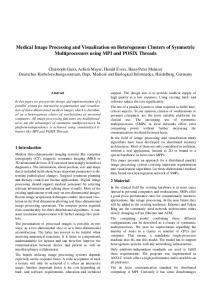
Figure 1. Visualization of a heterogeneous audio file.
Figure 2. Oscilloscope (left) and spectrogram (right) for a sound of cat meow.
1. INTRODUCTION Digital audio files are used widely in a variety of fields, such as film, television, computer gaming, radio, website design and audio book production. However, the query and navigation of audio files presents unique difficulties because of the linear nature of audio. There is considerable interest in making sound signals visible because the human visual system can rapidly scan a structured page of visual information, while sound files must be examined one by one, with each requiring a much longer period of the user’s attention. For example, scanning a set of 10 image mosaics representing audio files would require at most a few seconds, independent of the durations of the audio files they represent, while listening to each audio file sequentially would require the sum of the durations. Simply put, the objective of this work is to “view” what happens in the sound sequence. This project is a new approach to the visual representation of audio files as filtered mosaic time-line images. The resultant visualization is a composite image built from simple graphical elements driven by the audio data. The component images in the mosaics are individually retrieved for the sounds found in the given audio file, where the sounds are matched to audio in a pre-built audio-image database. The relative positions of image tiles in the resulting mosaic show the time sequences of their corresponding audio clips. In addition to identifying the component sounds, the visualization conveys more subtle audio features such as loudness, pitch, noise ratio,
etc, on a sound-by-sound basis. This is achieved by mapping audio properties to image filtering operations. Figure 1 shows a simple example that characteristically depicts the results that can be generated by this system. When given a heterogeneous audio file, each single sound is extracted and searched for in a pre-built audio-image database to determine what kind of sound it is. Then an image is generated based on its audio features and the template image that represents this kind of sound in the database. When all the images for the audio clips are generated, these images are combined together seamlessly according to the audio clips’ time sequences using a gradientdomain image compositing method. Using the resulting mosaics, the viewer is able to navigate amongst audio files. In addition, the viewer is able to ascertain certain audio features within the image results (e.g. noise ratio and power) at a glance, by the filtered component images. 2. RELATED WORK Sounds maybe visualized using existing methods such as oscilloscopes in time domain analysis and spectrograms in frequency domain analysis. The oscilloscope, as shown in Figure 2 (left), is
DAFX-1
Proc. of the 11th Int. Conference on Digital Audio Effects (DAFx-08), Espoo, Finland, September 1-4, 2008 a very common representation that expresses the audio signal by amplitude along a time axis. This might be considered the most direct visualization as it simply depicts the wave shape along the time axis. Conversely, a spectrogram represents the audio signal in the frequency domain, as shown in Figure 2 (right). The magnitudes of the windowed discrete-time Fourier transform are shown against the two orthogonal axes of time and frequency. For comparison, both Figure 2 (left) and (right) represent the same input sound of a cat’s meow. These visualizations are primarily targeted for scientific or quantitative analysis, and may not offer much insight for nonexpert and casual users. For example, it would be difficult if not impossible for most users to determine that the graphs (in Figure 2) represent a cat’s meow although they may be able to determine for example the average amplitude of the sound. Going beyond simple identification would be even more challenging. There are other visualizations that are derived from note-based or score-like representations of music, typically from MIDI note events [1]. Malinowski [2] introduced “The Music Animation Machine" (MAM), that displays the music's structure with bars of color representing the notes of the music. Smith and Williams [3] used standard music notation to visualize music by examining a note-based or score-like representation of a song. A trained musician may achieve an understanding of how a musical composition will sound but unfortunately, most people cannot read music in this way. More recently, Bergstrom, Karahalios and Hart [4] provided a new method for visualizing the structure of music. Viewers can grasp the music structure by a salient image of harmony as the music structure changes over time. All these methods are intended for knowledgeable users and are strictly designed to visualize musical sound. Audio segmentation is also related to the present work and is itself a widely researched topic. Commonly, a segmentation technique applies only to a specific application and cannot therefore be generalized. Some techniques are designed for audio samples that contain only one type of sound while others can be used for audio samples containing heterogeneous sound types. Existing methods can also be categorized into time-domain algorithms, frequency-domain algorithms or a hybrid of the two. These methods can also be further separated into supervised and unsupervised approaches depending on whether the system requires a training set to learn from, prior to audio segmentation. Segmentation approaches are also defined as model-based or non-model methods. The work of Panagiotakis and Tziritas [5] is a time-domain approach as it uses the root-mean-square (RMS) and Zero Crossing Rate (ZCR) to discriminate speech from music. Tzanetakis and Cook [6] present a general methodology for temporal segmentation based on multiple features. In model-based approaches, Gaussian mixture models (GMM) [7], [8], Hidden Markov Models (HMM) [9], Bayesian methods [10], and Artificial Neural Networks (ANN) [11] have all been applied to the task of segmentation. Unsupervised segmentation [12] and [10] does not require training sets but instead test the likelihood ratio between two hypotheses of change and no change for a given observation sequence. On the other hand, some systems must be trained before segmentation [9],[7]. Automatic audio classification offers ways to efficiently navigate audio databases and provide the necessary control for search and retrieval within those same databases. Sounds have been classified by genre [13], [14], [15], by mood or emotion [16],
[17], [18], [19], by instrumentation [20], or by segmentation and classification of an audio stream into speech, music, environmental sound and silence [21], [22]. There are many algorithms that have been applied to audio classification such as Nearest Feature Line [23], Rectified Nearest Feature Line Segment (RNFLS), Nearest Neighbour (NN), kNearest neighbor (k-NN), GMM, probabilistic neural network (PNN), Nearest Center (NC) and Support vector machines (SVMs) [24], [18]. A number of studies have been undertaken that compare the accuracy between these classification methods [24], [23], [25]. SVMs, together with a binary tree recognition strategy, a distance-from-boundary metric, and suitable feature combination selection, can obtain an error rate of 10% [24]. The Nearest Feature Line method has also been reported to achieve satisfactory accuracy (9.78% error) if a suitable feature combination is employed [23]. The present work defines a general method for audio visualization, which is more accessible than the existing methods because the filtered images used in the application are directly representative of sounds in the real world. 3. VISUALIZATION FRAMEWORK OVERVIEW Figure 3 shows the framework of our audio visualization system, which contains a pre-built audio-image database and three modules: Segmentation, Classification and Image Generation. The input to the system is a single audio file, which may contain a single sound or multiple sounds. The Segmentation module separates the input audio into audio clips, where each contains a single sound. Then each audio clip is classified by the Classification module, which retrieves the template images for the class that each audio clip belongs to. The Image Generation module then generates a distinctive image based on the computed audio features found in the sound clip and its class template image. The output of the system is an image mosaic, which is composed of all images produced by the Image Generation module, according to the sequence order and duration of audio clips. From the mosaic viewers can determine what sounds exist within a given audio file and can scan visual cues which help the user to determine each clip’s audio features.
DAFX-2
Figure 3. Framework of the audio visualization system.
Proc. of the 11th Int. Conference on Digital Audio Effects (DAFx-08), Espoo, Finland, September 1-4, 2008 benchmark. However, Muscle Fish is not entirely suitable for our application because some of the audio files are too broadly classified. In the “animals” class, for example, there are 9 sounds that belong to 6 different kinds of animal namely: cats (kittens), chickens, dogs, ducks (and geese), horses and pigs. Such a set cannot be meaningfully represented by single archetypical template image. Therefore in order to fully test our time mosaic generation we built a new database named VisualData (in Table 2) that is based on the Muscle Fish database. The VisualData training set has 602 audio files classified at a more suitable granularity. A discussion of our experiments based on these databases is discussed in the following section. Input Audio
Figure 4. A class in the database.
Audio Feature Extraction
3.1. The Audio-Image Database The audio-image database is a key component of the system. Sets of audio-image pairs are stored in the database, together with their classification and training information. This comprises a library that associates sounds with archetypal images. Figure 4 illustrates a class in the database where each class, based upon a fixed and pre-determined ontology, contains a single manually chosen template image, shown top-left. The remaining images that are associated with each audio file in the class are automatically generated by the system based on the template and each file’s audio properties. The differences in audio features between the audio files in a class determine the different visual features of their corresponding images. As new audio files are added to the database, the audio is analyzed and a new representative image is produced. A set of audio files known as the “Muscle Fish” database is widely used as a standard non-musical sound database for the development of audio matching and classification algorithms [26], [23]. There are 16 classes and 410 audio files in the Muscle Fish database, as described in Table 1, with Nc being the number of sounds in each class. The performance of the Segmentation and Classification modules were initially evaluated using the Muscle Fish database as a Table 1 & 2: MuscleFish and VisualData Ontological Structures Muscle Fish Classes Alto trombone Animals Bells Cello (bowed) Crowds Female Voice Laughter Machines Male Voice Oboe Percussion Telephone Tubular Bells Volin (bowed) Volin (pizz) Water Total
Nc 13 9 7 47 4 35 7 11 17 32 99 17 20 45 40 7 410
VisualData Class Bee Bell Bird Cat Cow Duck Dog Frog Rooster Alto trombone Cello (bowed) Oboe Tubular Bells Volin (bowed) Volin (pizz) Telephone Total
Nc 36 14 15 45 79 15 13 99 23 13 47 32 20 45 40 66 602
Clip-Based End Point Detection
Frame-Based
Audio Feature Extraction
Frequency Domain Similarity Output Clips
Figure 5. Segmentation module framework.
Figure 6. Segmentation result for long and short signals. 4. AUDIO SEGMENTATION AND CLASSIFICATION The first module in our system pre-processes the input audio and performs any required segmentation. The goal of the audio segmentation process is to determine the beginning and ending positions (end-points) for each sound if there is no overlap between the connected audio clips. Where overlapping regions exist, the goal becomes the identification of the overlapping areas between the connected audio clips. General audio files may have a short period of silence between sounds in the cases where sound clips do not overlap. Therefore silence detection can often be used to separate sounds in the same file. Alternatively, when we cannot rely on the presence of silence, we require a more sophisticated approach to separation of the sound clips. Because a sound tends to be homogeneous, in terms of its audio features, any abrupt changes in audio features may indicate the start of a new sound clip. We can therefore exploit time-domain features to detect silences, and then use frequency domain features to separate any remaining sound clips. Figure 5 shows the stages of this segmentation process. Our segmentation method is designed for both long and short duration clips. Figure 6 shows results obtained by our segmentation module. In this example, there are 5 audio clips. The 1st and
DAFX-3
Proc. of the 11th Int. Conference on Digital Audio Effects (DAFx-08), Espoo, Finland, September 1-4, 2008 5th have a relatively long duration and the rest are relatively short. The resulting segmentation is demarked with red lines over the original waveform. After segmentation a series of sound clips has been generated where each sound clip is a segment of audio, containing a homogeneous set of features for each frame. Once segmentation has been achieved and the set of audio clips has been determined, each clip is then classified and subsequently stored in the database using the classification module (Figure 3). This module is concerned with determining the clips classification based on a comparison of existing sound files in the database using extracted audio features. It is important to obtain an accurate classification in order for the visualization to be meaningful. For each audio clip output from the segmentation module, a Nearest Feature Line (NFL) based classification is performed which has been reported to give the best classification results to date for audio file classification [6]. In this classification method an audio feature set is extracted which is composed of the means and standard deviations of the Total Spectrum Power, Subband Power, Brightness, Bandwidth and Pitch, as well as 8 order Mel Frequency Cepstral Coefficients (MFCCs). Details on the computation of these features can be found in [6]. This feature set is then used to determine which class an audio file is closest to and should belong to. Our experiments using both the MuscleFish and the VisualData databases, achieved a similar accuracy for classification and segmentation. Using the Muscle Fish data we achieved a 90% accuracy of classification and using the VisualData set we achieved a similar result of 91%. All matching results in this paper were obtained using leave-one-out cross-validation. The classification system we have developed is currently being extended so that it is capable of identifying new classes of audio files. However, a full discussion of our adapted NFL algorithm and evolving classification system for audio files is outside the scope of this paper and is to be published elsewhere. 5. IMAGE TILE GENERATION Following audio segmentation and classification, the template images in the database are used to visualize the characteristics of the input audio. The function of this module is to generate images that clearly represent the embedded audio clips, while incorporating as many useful audio features as possible in the form of image filters. Our system computes 36 audio features in order to perform analysis, segmentation and classification. Some of these features such as pitch and power are easily perceived by humans while others which have no metaphorical analogues in human audio perception are strictly used for audio analysis such as bandwidth and MFCCs. We therefore map only a subset of these audio features to image filtering operations. The image processing operations are sufficient to produce distinctive images for individual audio files within the same class.
1) Power is perhaps the simplest feature of an audio clip. It is related to the perceived loudness of a sound. The higher the volume (amplitude), the higher the power of the audio, and the louder a human will understand it to be. 2) Pitch is another feature that listeners can readily comprehend. In the field of music analysis, pitch perception is often thought of in two dimensions, pitch height and pitch chroma [27]. But for casual users, it may be sufficient to know that an audio clip with a high pitch sounds high and shrill, while low pitched sound is deep and soft [28]. Acoustics research indicates that pure sinusoids sound sharp and very low frequencies sound flat, compared to a purely logarithmic relationship [29]. As our aim is to let viewers grasp the difference between pitches by a glance, we need only visualize differences within classes. The precise values of the pitches are not required. 3) The Signal-to-Noise Ratio (SNR) can also be understood by the human ear. We understand it as the clarity of the signal. For example, poorly recorded audio, or audio with significant background noise will have a low signal-to-noise ratio. Correspondingly, there are visual features that may be mapped to the described audio features, such as image brightness and contrast, the color-depth and signal-to-noise ratio in an image. 5.2. Mapping Audio Features to Visual Features We map the audio features to a set of image processing operations as shown in the legend in Figure 7. These are the systems default audio-to-visual feature mapping, though it would be trivial to allow the user to explicitly over-ride the default mapping with his or her preferences. We first describe the mappings in general terms before defining them explicitly. The top row illustrates how the audio SNR affects the visual noise ratio. The blue signal under the row of images denotes the pure audio signal for each sound clip. The red wrapping around the signal denotes noise added to the clear audio signals with varying degrees of white Gaussian noise added. The audio files generated become increasingly “noisy” from left to the right with the far left image representing the pure starting audio file and, accordingly, the images become noisier to represent this change in the signal to noise ratio of the input audio file. Brightness values for the template image are also linearly scaled to fit the pitch of an input audio as is shown in the second row of Figure 7. The template image represents an audio clip with the average pitch of the class. The audio sounds high and
5.1. Interpretable Audio Features There are many audio features that relate to the way humans perceive sound, such as pitch, power and signal-to-noise ratio. Here we are visualizing such features so that viewers can grasp the character of the audio. We now discuss each of the audio features that we have incorporated:
DAFX-4
Figure 7. Legend of visualized audio features.
Proc. of the 11th Int. Conference on Digital Audio Effects (DAFx-08), Espoo, Finland, September 1-4, 2008 then calculated as Ioutput=I×Brightness, with the adjustment made within HSV color space. 5.2.3. Calculating the color depth parameter The ColorDepth scale is calculated in 3 stages: Figure 8. Algorithm to represent the audio noise ratio. shrill when the pitch is high, so the image is set to be brighter for such sounds and darker for lower pitched ones. The pitch comparison is strictly within classes. For example, the pitch of a bees’ buzz is always higher than an oboe’s sound, but it would not convey additional information to set the brightness of bees to always be very high and the brightness of oboes to be always very dark. Therefore, the visual representation of pitch is made to be relative within the same class, meaning that the viewer can interpret a bright picture of a dog as being a relatively high pitched dog bark. Power represents the degree of “loudness” or the volume of a sound. The higher the power value, the more clearly it can be sensed. We have chosen to map the power of an audio clip to the color depth of the image. The metaphor employed to illustrate this is that as a sound’s power fades, so does the color in an image. The 3rd row of Figure 7 shows this relationship. In addition to the above relationships, the size of an image is used to represent the duration of the audio as shown in the lowest row of Figure 7. Suppose the template image I represents class A, which audio clip a belongs to. The database contains all audio clips Ai belonging to the same class A and their audio features we r denote as Avi . The audio features for the given audio clip
r
are av . The steps of generate an image Ioutput for given audio a are detailed in the following subsections.
1)
The audio clip is normalized to set the maximum of amplitude value equal to 1, producing Normal(a). Then the power → value is calculated as max avpower.
2)
Normal(a) is scaled to 0.01×Normal(a) calculate the power → value as min avpower. This value is chosen empirically given that small amplitude is not easily heard by the human ear.
3)
The color depth ranges from a maximum of 28 to a minimum of 22. The color depth scale is calculated as: 2 +6 ×
ColorDepth = 2
→
→
5.2.4. Representing the audio noise-to-signal ratio We designed three algorithms for representing different levels of Noise-to-Signal Ratios (NSR) from very clean to very noisy, as shown in Figure 8. Note that aNSR is the NSR for audio clip a. To represent the NSR of a given audio, not only is independent Gaussian noise added to the template image, but also white point noise for very noisy audio files. Furthermore, a degree of blurring is introduced for extremely noisy audio files. Each of the three filtering processes is calculated as follows: 1)
→
⎧ 0.75 × ( avr pitch − medianAvr pitch ) ⎪ max Avr pitch − medianAvr pitch Brightness = ⎨ r r 0.75 × ( medianAv pitch − av pitch ) ⎪ r r ⎩ medianAv pitch − min Av pitch →
if
Independent white Gaussian noise is added to Ioutput. If aNSR is less than the maximum NSR maxANSR in the class it belongs to, it is the only form of visual noise that is added. The white Gaussian noise is zero-mean, with a variance of: NoiseScale =
2)
r av NSR 0.15 × max avr NSR
3)
(3)
After adding independent white Gaussian noise, white points are added when aNSR is between 1 to 1.5 times maxANSR. The number of white points is defined by: PointNumber = 0.1 ×
5.2.2. Calculating the brightness scale parameter The brightness of the template image is used as the standard to represent the median pitch of a class. When the pitch of the given audio is higher than the median pitch of the class, the resulting image is brighter than the template image. For the audio with pitch lower than the median pitch of the class, the resulting image is darker than the template. The brightness is calculated as follows:
(2)
A new index image, Ioutput, is generated by using minimum variance quantization on ColorDepth as calculated in sect. 5.2.2. The number of colours in the new index image is at most ColorDepth.
5.2.1. The Audio-Image Database The audio features we used are avpitch, avpower, avNSR and its duration. Signal-to-noise ratio is a concept defined as the ratio of a signals power to the noise power corrupting the signal. It compares the level of a desired signal (such as music) to the level of background noise. The higher the ratio, the less obtrusive the background noise is. Here we use its inverse (Noise-signal-ratio) → avNSR to represent the noise level of the background to audio.
r r av power − min av power r r max av power − min av power
r r av SNR − max Av NSR r 0.5× max Av NSR
(4)
The image is blurred with 7 * 7 Gaussian low-pass filter if aNSR is larger than 1.5 * maxANSR.
Together, the three filters introduce a wide range of noise distortion in the final image.
r r av pitch ≥ medianAv pitch
(1) otherwise →
Where avpitch, is the pitch value of audio clip a; medianAvpitch, → → maxAvpitch, and minAvpitch, are the median, maximum and minimum values of the pitch values in class A. The adjusted image is
DAFX-5
Figure 9. Background texture generation.
Proc. of the 11th Int. Conference on Digital Audio Effects (DAFx-08), Espoo, Finland, September 1-4, 2008 5.2.5. Resizing the output image by audio duration Image size is used to represent the duration of the audio clip. The longer the audio lasts, the larger its image size. In order to be able to display multiple timeline mosaics simultaneously, we set maximum width of component images to 512 and the smallest to 128 pixels. If the duration r of a givenr audio is less than all the audio files in its class av duration ≤ min Av duration , the width of its image tile is set to 128 to make sure the image is sufficiently clear. When the duration of a given audio clip is longer than all audio files, then the image is set to 512. Otherwise, the image size is scaled linearly between the smallest and largest size based on the audio’s duration. After these five stages, an image tile is generated to represent the given audio clip. All the image tiles are generated independently. 5.3. Mosaic Time-Line Generation It is not practical to assume that all audio clips have the same length in a general audio file. Constructing a blended image mosaic is therefore appropriate since the image sizes will vary, given that embedded audio clips are of varying lengths. Blended image mosaics solve this problem since we can embed smaller images into a larger image background. Poisson image editing [30] is an effective approach for seamless image composition in the gradient domain. The new image is created by pasting a region from a source image onto a target image. To construct a time-line mosaic from the component images Poisson image editing [30] is employed to fuse the separate images together without significantly altering the content of each region. The optimization process seamlessly inserts new content into a subset, Ω, of an existing image, h. It computes a new image, f, whose gradient, f, within Ω is closest to the gradient g, taken from a second image, g. The original boundary, ∂Ω, of region Ω from h is also used as a constraint to ensure that the region Ω blends with the surrounding image, h. The final image constrains an interpolation of the boundary conditions, ∂Ω, inwards while conforming to the spatial changes of the guidance field from g as closely as possible within Ω. The minimization problem is written as: min f
∫∫ ∇f Ω
− ∇g
2
with f
∂Ω
= h ∂Ω
(5)
The reader is directed to [30] for the discretization of the problem and for suggested iterative solvers. For our application, the output image is generated based on rectangular images of different sizes. The challenge is to merge different-size images without significant information loss in any of the component images that form the final mosaic. When the image tiles within the same mosaic are not the same size, this creates gaps in the mosaic at the top and bottom of the smaller tiles, which must be padded in an unobtrusive way. To achieve this we follow the stages depicted in Figure 9 to generate the final image. In this mosaic there are three tiles (A, B and C). Tile A does not require padding and is placed directly into the output mosaic. Tiles B and C are smaller and require varying degrees of padding. For this, the largest tile (A) is selected to generate a seamless background texture to pad the smaller tiles. As most of the important information within our archetypal images is in the center, we conservatively scale padding image A to 90% of its original size and integrate the result into the original
tile A with Poisson blending to generate additional, low-content padding. This process repeats 10 times until the final image A* has the same size as the original image A, but with its content comprised of edges from the original image. The width of the background texture image A* is then scaled to fit the width of each image tile (see note (2) in Figure 9). The A1* is used for the background texture for image B and the A2* is used for C. Tile B is then merged into the middle of A1* with Poisson blending to generate image tile B’. When all the image tiles are padded, they are merged seamlessly by Poisson image editing in order of their time sequences. 6. EXPERIMENTAL RESULTS We now discuss a set of experimental results. The input audio of the first example includes a long bird’s sound, 3 short dog barks and a relatively long cat’s meow, as shown in different colors in the bottom of Figure 10. Note that the power or amplitude of the sounds cannot be read directly from the signal at the bottom of Figure 10 because the audio clips are normalized to show their shapes. This is necessary for audio clips with small amplitudes. After segmentation, the input audio file is separated into 5 audio clips each containing only one sound. The three dog’s barks are separated into 3 clips each containing only one sound. After classification, we know which classes the audio clips belong to, and have the template images for each audio clip. A result generated based on these template images is shown in Figure 10. This result indicates what sounds are included in the given audio file, their duration, but have not been subjected to image filtering. Figure 11 is a result generated based on both the template image and the audio features of each audio clip. Comparing Figure 10 (without filtering) and Figure 11 (with filtering) we can see that the cat meow in the given audio is very noisy because the tile is quite noisy and blurry. The noise ratio of dog’s sound is lower compared with the cat’s sound and the sound of the bird has the lowest noise ratio of the three. According to the legend in Figure 7, from the ColorDepth and brightness in the Figure 11, we can read that the power of the bird’s sound is relatively low and its pitch is relatively high compared with most audio files in the same class. Comparing Figures 11 and 12, one can easily determine information such as which audio clip is noisier, which has a higher pitch and which has more power value. Figures 13 and 14 show two further examples of randomly generated audio files, and Figure 15 shows an example with 5 detected sound clips. Figure 17 gives an example for random generated audio for music, which contains 3 music clips: oboe, trombone and violin.
DAFX-6
Figure 10. Bird-dog-cat example without filtering.
Proc. of the 11th Int. Conference on Digital Audio Effects (DAFx-08), Espoo, Finland, September 1-4, 2008
Figure 16. Bird-dog-cat example with alternate template images.
Figure 11. Bird-dog-cat example with filtering.
Figure 17. Oboe-trombone-violin. 7. LIMITATIONS
Figure 12. Filtered bird-dog-cat example with different features.
Figure 13. Frog-telephone-rooster example.
Figure 14. Bee-Cow-Rooster example.
Figure 15. Results with 5 images.
There remain some limitations of our system, which may lead to spurious results under certain conditions. The template images of the database partly determine the quality of the final result. The requisites for a good template image include: the color and contrast of the image, the position of important information and whether the image can completely describe the class it represents. Figure 16 is an image result for the same sound but with different template images for the classes in VisualData. In this result, because the most important information (the dog) of the template image of class “dog bark” is very close to the left edge, part of the audio clip is not clearly represented. The accuracy of visualizing a given sound with time mosaics also depends on the quality of the pre-built database, the accuracy of audio segmentation and classification. If given a sound which contains any audio clip doesn’t belong to any class of the database, the system cannot recognize it and does not yet have the ability to notify the user about the accuracy of audio segmentation and classification. However, as noted previously, we are currently augmenting our system to handle this issue. Figure 18 illustrates a limitation in our audio processing method. The sound file contains a cat-bird-dog sequence of sounds. The bird sound in this file has amplitude that is too low for our segmentation method to detect and results in a time mosaic with only 2 component images. If the amplitude of the bird sound in this file is increased by a factor of 2 then our segmentation method detects the bird sound and accurately produces a time mosaic with 3 component images (Figure 19) Another possible source of error can occur in situations where sounds overlap. Figure 20 shows an audio signal that consists of a cat’s meow and a bird sound in which there is a period of overlap between them. The segmentation failed to separate the 2 sounds, resulting in the sound file being treated as a single sound and classified as a rooster for which a single image was produced.
DAFX-7
Proc. of the 11th Int. Conference on Digital Audio Effects (DAFx-08), Espoo, Finland, September 1-4, 2008 [8] [9]
[10]
Figure 18. Three sounds misrepresented as two images.
[11]
[12]
Figure 19. Three sounds correctly represented as three images. [13]
[14]
[15] [16]
Figure 20. Overlapping audio signals producing an incorrect result.
[17]
8. CONCLUSIONS AND FUTURE WORK
[18]
This paper presents a novel approach to visualizing a given audio file with time mosaics, constructed from a pre-built audio database. The mosaics provides produce a sequence of images seamlessly joined together using the Poisson image editing method. Each filtered image tile in the mosaic represents a single monophonic sound and its features, in the given input audio. We argue that the system would provide a useful means to quickly scan audio query results and navigate an audio database. There are a number of opportunities to further develop the ideas introduced in this paper. For example, the concept of time mosaics could be extended and used as a basis for generating video to represent sound files. Other mapping from audio features to image processing filters could also be explored, including NPR filters. 9. REFERENCES [1] [2] [3] [4] [5]
[6]
[7]
[19]
[20]
[21]
[22]
[23]
[24]
J. Foote. Visualizing Music and Audio using Self-Similarity. In International Multimedia Conference, pp 77-80, 1999. S. Malinowski. Music Animation Machine. 2007 [cited; Available at: http://www.well.com/user/smalin/mam.html]. S.M. Smith and G.N. Williams. A Visualization of Music. In Proc. Visualization '97, ACM, pp 499-503. 1997. T. Bergstrom, K. Karahalios and J. Hart. Isochords: Visualizing Structure in Music. Graphics Interface, pp: 297-304, 2007. C. Panagiotakis and G. Tziritas. A Speech/Music Discriminator Based on RMS and Zero-Crossings. IEEE Transactions on Multimedia, Volume 7, pp 155-166. July, 2004. G. Tzanetakis and P. Cook. Multifeature Audio Segmentation for Browsing and Annotation. In IEEE Workshop on Applications of Signal Processing to Audio and Acoustics, pp 103-106, 1999. M. Spina and V. Zue. Automatic transcription of general audio data: preliminary analyses. In Spoken Language, pp 594-597, 1996.
[25] [26]
[27] [28] [29]
[30]
DAFX-8
H. Aronowitz. Segmental Modeling for Audio Segmentation. In Acoustics, Speech and Signal Processing, pp 393-396, 2007. B. Ramabhadran, J. Huang, U. Chaudhari, G. Iyengar and H.J. Nock. Impact of audio segmentation and segment clustering on automated transcription accuracy of large spoken archives. In Proc. EuroSpeech, pp 2589-2592, 2003. S. Chen and P. Gopalakrishnan. Speaker Environment and Channel Change Detection and Clustering via The Bayesian Information Criterion, DARPA speech recognition workshop, pp 679-682. H. Meinedo and J. Neto. A Stream-based Audio Segmentation, Classification and Clustering Pre-processing System for Broadcast News using ANN Models. In INTERSPEECH, pp 237-240, 2005. M.K. Omar, U. Chaudhari and G. Ramaswamy. Blind Change Detection for Audio Segmentation. In Acoustics, Speech, and Signal Processing, pp 501-504, 2005. Z. Cataltepe, Y. Yaslan and A. Sonmez. Music Genre Classification Using MIDI and Audio Features. EURASIP Journal on Advances in Signal Processing, pp 150-157, 2006. S. Lippens et al. A comparison of human and automatic musical genre classification. In IEEE International Conference on Audio, Speech and Signal Processing, volume 4, pp 233-236, 2004. M.F. McKinney and J. Breebaart. Features for audio and music classification. ISMIR, pp 151-158, 2003. Y. Feng, Y. Zhuang and Y. Pan, Popular music retrieval by detecting mood. SIGIR, pp 375-376, 2003. L. Lu, D. Liu and H.-J. Zhang. Automatic Mood Detection and Tracking of Music Audio Signals. IEEE Transactions On Audio, Speech, And Language Processing, pp 5-18. M. Mandel, G. Poliner and D.Ellis. Support vector machine active learning for music retrieval. Multimedia Systems, 12, pp 3-13. T. Pohle, E. Pampalk and G. Widmer. Evaluation of Frequently Used Audio Features for Classification of Music into Perceptual Categories. Proceedings of the 4th International Workshop on Content-Based Multimedia Indexing, 2005. S. Essid, G. Richard and B. David. Musical instrument recognition by pairwise classification strategies. IEEE transactions on audio, speech and language processing, pp 1401-1412, 2006. S. Kiranyaz, A. Qureshi and M. Gabbouj. A Generic Audio Classification & Segmentation Approach for Multimedia Indexing & Retrieval. Audio, Speech and Language Processing, 14, pp 1062-1081. L. Lu, H. Jiang and H. Zhang. A robust audio classification and segmentation method. In 9th ACM international Conference on Multimedia, MULTIMEDIA '01, pages 203-211, 2001. S.Z. Li. Content-based audio classification and retrieval using the nearest feature line method. IEEE transactions on speech and audio processing, volume 8, pp 619-625, 2000. G. Guo and S.Z. Li. Content-based audio classification and retrieval by support vector machines. In Neural Networks, IEEE Transactions on, pp 209-215, 2003. M. Liu and C. Wan. Feature Selection for Automatic Classification of Musical Instrument Sounds. ACM, pp 247-248, 2001. E. Wold, T. Blum, D. Keislar and J. Wheaton. Content-Based Classification, Search, and Retrieval of Audio. Multimedia, IEEE, volume 3, pp 27-36, 1996. R. Shepard. Circularity in Judgments of Relative Pitch. The Journal of the Acoustical Society of America, 36(12), pp 2346-2353. H.W. Lie, P.E. Dybvik and J. Rygh. SCREAM: screen-based navigation in voice messages. In Visual Languages, pp 401-405, 1993. S. Coren, L.M. Ward and J.T. Enns. Sensation and Perception. 1994: Harcourt Brace College Publisher, Toronto. P. Perez, M. Gangnet and A. Blake. Poisson Image Editing. In International Conference on Computer Graphics and Interactive Techniques (ACM SIGGRAPH 2003), pp 313-318.