An Implementation Of The Annis 2 Query Language Viktor Rosenfeld∗ Supervisor: Ulf Leser April 23, 2010 We describe the Annis 2 Query Language and show how its features including operations on distinct graphs over the same nodes can be implemented using a relational database as a back-end. We provide a reference implementation on top of PostgreSQL and measure its performance on consumer hardware.
∗
[email protected]
Contents 1 Introduction 1.1 Historical overview of Annis . . . . . . . . . . . . . . . . . . . . . . . . . . . . . . . . . . . 1.2 Goals and structure of this work . . . . . . . . . . . . . . . . . . . . . . . . . . . . . . . .
5 5 6
2 Corpus Data Model 2.1 Overview . . . . . . . . . . . . . . . . . . . . . . . . . . . . . . . . . . . . . . . . . . . . . 2.2 Key concepts . . . . . . . . . . . . . . . . . . . . . . . . . . . . . . . . . . . . . . . . . . . 2.3 SQL schema . . . . . . . . . . . . . . . . . . . . . . . . . . . . . . . . . . . . . . . . . . . .
7 7 7 8
3 Annis 2 Query Language 3.1 Introductory example . . . . . . . . . . . . . 3.2 Text span search terms . . . . . . . . . . . . . 3.3 Linguistic constraints . . . . . . . . . . . . . . 3.3.1 Coverage . . . . . . . . . . . . . . . . 3.3.2 Dominance . . . . . . . . . . . . . . . 3.3.3 Precedence . . . . . . . . . . . . . . . 3.3.4 Pointing relations . . . . . . . . . . . . 3.3.5 Text span constraints . . . . . . . . . 3.4 Combining expressions with OR . . . . . . . . 3.5 Meta data . . . . . . . . . . . . . . . . . . . . 3.6 Query evaluation . . . . . . . . . . . . . . . . 3.7 Query functions . . . . . . . . . . . . . . . . . 3.8 Pagination of AN N OT AT E results . . . . . 3.9 Differences between ANNIS-QL 1 and AQL2
. . . . . . . . . . . . . .
. . . . . . . . . . . . . .
. . . . . . . . . . . . . .
. . . . . . . . . . . . . .
. . . . . . . . . . . . . .
. . . . . . . . . . . . . .
. . . . . . . . . . . . . .
. . . . . . . . . . . . . .
. . . . . . . . . . . . . .
. . . . . . . . . . . . . .
. . . . . . . . . . . . . .
. . . . . . . . . . . . . .
. . . . . . . . . . . . . .
. . . . . . . . . . . . . .
. . . . . . . . . . . . . .
. . . . . . . . . . . . . .
. . . . . . . . . . . . . .
. . . . . . . . . . . . . .
11 11 12 12 12 12 14 14 15 15 16 16 17 18 18
4 SQL Generation 4.1 Computation of derived node data during corpus import . . 4.1.1 Minimally and maximally covered tokens . . . . . . 4.1.2 Root nodes in the original ODAG . . . . . . . . . . 4.1.3 Identification of a node’s top-level corpus . . . . . . 4.2 The SELECT and FROM clauses . . . . . . . . . . . . . . . 4.3 The WHERE clause: Translation of AQL2 language features 4.3.1 Text search . . . . . . . . . . . . . . . . . . . . . . . 4.3.2 Token search . . . . . . . . . . . . . . . . . . . . . . 4.3.3 Annotation search . . . . . . . . . . . . . . . . . . . 4.3.4 Node search . . . . . . . . . . . . . . . . . . . . . . . 4.3.5 Coverage . . . . . . . . . . . . . . . . . . . . . . . . 4.3.6 Precedence . . . . . . . . . . . . . . . . . . . . . . . 4.3.7 Dominance and pointing relations . . . . . . . . . . 4.3.8 Root nodes . . . . . . . . . . . . . . . . . . . . . . . 4.3.9 Node arity . . . . . . . . . . . . . . . . . . . . . . . 4.3.10 Token arity . . . . . . . . . . . . . . . . . . . . . . . 4.4 Query alternatives . . . . . . . . . . . . . . . . . . . . . . . 4.5 Corpus selection . . . . . . . . . . . . . . . . . . . . . . . . 4.6 Meta data filtering . . . . . . . . . . . . . . . . . . . . . . . 4.7 Query functions . . . . . . . . . . . . . . . . . . . . . . . . . 4.7.1 The COU N T function . . . . . . . . . . . . . . . . . 4.7.2 The AN N OT AT E function . . . . . . . . . . . . . . 4.7.3 The M AT RIX function . . . . . . . . . . . . . . . .
. . . . . . . . . . . . . . . . . . . . . . .
. . . . . . . . . . . . . . . . . . . . . . .
. . . . . . . . . . . . . . . . . . . . . . .
. . . . . . . . . . . . . . . . . . . . . . .
. . . . . . . . . . . . . . . . . . . . . . .
. . . . . . . . . . . . . . . . . . . . . . .
. . . . . . . . . . . . . . . . . . . . . . .
. . . . . . . . . . . . . . . . . . . . . . .
. . . . . . . . . . . . . . . . . . . . . . .
. . . . . . . . . . . . . . . . . . . . . . .
. . . . . . . . . . . . . . . . . . . . . . .
. . . . . . . . . . . . . . . . . . . . . . .
. . . . . . . . . . . . . . . . . . . . . . .
. . . . . . . . . . . . . . . . . . . . . . .
. . . . . . . . . . . . . . . . . . . . . . .
. . . . . . . . . . . . . . . . . . . . . . .
. . . . . . . . . . . . . . . . . . . . . . .
20 20 20 20 21 21 21 21 22 22 23 23 23 24 29 29 29 30 30 31 32 32 32 32
. . . . . . . . . . . . . .
. . . . . . . . . . . . . .
. . . . . . . . . . . . . .
. . . . . . . . . . . . . .
. . . . . . . . . . . . . .
. . . . . . . . . . . . . .
. . . . . . . . . . . . . .
5 Related work 34 5.1 TIGERSearch . . . . . . . . . . . . . . . . . . . . . . . . . . . . . . . . . . . . . . . . . . . 34
2
5.2
Evaluating XPath queries using relational databases . . . . . . . . . . . . . . . . . . . . . 35
6 Evaluation and Optimization 6.1 Search boundaries for ranged operators . . . . . . . . . . . . . . . . . 6.2 Performance of the normalized corpus data model . . . . . . . . . . . 6.3 The materialized facts table . . . . . . . . . . . . . . . . . . . . . . . 6.4 Combined node lookup and node join . . . . . . . . . . . . . . . . . 6.4.1 Indexed attributes for search terms and linguistic constraints 6.4.2 Partial indexes . . . . . . . . . . . . . . . . . . . . . . . . . . 6.4.3 Evaluation of different indexing strategies . . . . . . . . . . . 6.5 The M AT RIX query function . . . . . . . . . . . . . . . . . . . . . 6.6 The AN N OT AT E query function . . . . . . . . . . . . . . . . . . . 6.7 Rewriting queries with anchored regular expression searches . . . . . 6.8 Influence of document size . . . . . . . . . . . . . . . . . . . . . . . .
. . . . . . . . . . .
. . . . . . . . . . .
. . . . . . . . . . .
. . . . . . . . . . .
. . . . . . . . . . .
. . . . . . . . . . .
. . . . . . . . . . .
. . . . . . . . . . .
. . . . . . . . . . .
. . . . . . . . . . .
. . . . . . . . . . .
. . . . . . . . . . .
36 36 38 38 39 42 43 43 44 46 47 48
7 Conclusions and Outlook
50
A Annis 2 Query Language Grammar
52
B Internal DDDquery implementation 54 B.1 Supported DDDquery features and custom extensions . . . . . . . . . . . . . . . . . . . . 54 B.2 Mapping from AQL2 to DDDquery . . . . . . . . . . . . . . . . . . . . . . . . . . . . . . . 55 C SQL Schema of the Corpus Data Model D Experimental Setup D.1 Test queries . . . . . . . . . . . . D.2 The Tiger corpus . . . . . . . . D.3 Test system . . . . . . . . . . . . D.4 PostgreSQL configuration . . . . D.5 Configuration of system resources
. . . . .
. . . . .
57
. . . . .
. . . . .
. . . . .
. . . . .
. . . . .
. . . . .
. . . . .
. . . . .
. . . . .
. . . . .
. . . . .
. . . . .
. . . . .
. . . . .
. . . . .
. . . . .
. . . . .
. . . . .
. . . . .
. . . . .
. . . . .
. . . . .
. . . . .
. . . . .
. . . . .
. . . . .
. . . . .
. . . . .
. . . . .
. . . . .
References
59 59 59 61 61 61 63
List of Figures 1 2 3 4 5 6 7 8 9 10 11 12 13 14 15 16 17 18 19
Screenshot of the Annis 2 web application . . . . . . . . . . . . . . . . . . . . . . . . . . . Relational schema of the corpus data model. . . . . . . . . . . . . . . . . . . . . . . . . . . A match from the PCC3 corpus for the query example. . . . . . . . . . . . . . . . . . . . Syntax tree fragment demonstrating different dominance relationships between spans. . . Annotation graph fragment demonstrating different precedence relationships between spans. Using pointing relations to model information structure. . . . . . . . . . . . . . . . . . . . Annotation graph with pointing relations and multiple syntax trees. . . . . . . . . . . . . Annotation graph partitioned by edge type. . . . . . . . . . . . . . . . . . . . . . . . . . . Annotation graph partitioned by edge type and name. . . . . . . . . . . . . . . . . . . . . Annotation graph components for each combination of edge type and name. . . . . . . . . Effect of the inclusion optimization. . . . . . . . . . . . . . . . . . . . . . . . . . . . . . . Join plan generated by PostgreSQL for query 9. . . . . . . . . . . . . . . . . . . . . . . . . Performance of COU N T on the normalized source tables and the materialized facts table. Execution plan generated by PostgreSQL for query 5 with nested loops joins enabled. . . Execution plan generated by PostgreSQL for query 5 with nested loops joins disabled. . . Comparison of average vs. best runtime. . . . . . . . . . . . . . . . . . . . . . . . . . . . . Evaluation time of the M AT RIX query function. . . . . . . . . . . . . . . . . . . . . . . Influence of limit and context on AN N OT AT E. . . . . . . . . . . . . . . . . . . . . . . . Comparison of COU N T vs. AN N OT AT E. . . . . . . . . . . . . . . . . . . . . . . . . . .
3
5 9 11 14 15 15 24 25 26 27 37 38 39 40 41 45 45 46 47
20 21 22 23 24
Execution plan for unanchored regular expression searches. . . . . . . . . . . . Execution plan for anchored regular expression searches. . . . . . . . . . . . . . Performance of unanchored vs. anchored regular expressions. . . . . . . . . . . Comparison of average vs. best runtime on the 1 GB Tiger instance. . . . . . Best runtime in five sequential runs on the 500 MB and 1 GB Tiger instances.
. . . . .
. . . . .
. . . . .
. . . . .
. . . . .
. . . . .
47 48 48 49 49
. . . . . . . . . . . . . . . . . . . . . . .
. . . . . . . . . . . . . . . . . . . . . . .
. . . . . . . . . . . . . . . . . . . . . . .
. . . . . . . . . . . . . . . . . . . . . . .
. . . . . . . . . . . . . . . . . . . . . . .
. . . . . . . . . . . . . . . . . . . . . . .
. . . . . . . . . . . . . . . . . . . . . . .
12 13 13 14 15 16 37 39 42 43 44 44 46 46 55 55 56 59 59 60 60 60 62
FROM clause generated for an Annis query. . . . . . . . . . . . . . . . . . . . . SQL query template for Annis queries with multiple alternatives using UNION. SQL query for the AN N OT AT E function. . . . . . . . . . . . . . . . . . . . . Table definitions for the SQL schema of the corpus data model. . . . . . . . . . PostgreSQL configuration . . . . . . . . . . . . . . . . . . . . . . . . . . . . . .
. . . . .
. . . . .
. . . . .
. . . . .
. . . . .
. . . . .
22 31 33 57 61
List of Tables 1 2 3 4 5 6 7 8 9 10 11 12 13 14 15 16 17 18 19 20 21 22 23
Coverage operations in AQL2. . . . . . . . . . . . . . . . . . . . . . . . . . Possible coverage relationships between spans. . . . . . . . . . . . . . . . . Dominance operations in AQL2. . . . . . . . . . . . . . . . . . . . . . . . Precedence operations in AQL2. . . . . . . . . . . . . . . . . . . . . . . . Pointing relation operations in AQL2. . . . . . . . . . . . . . . . . . . . . Unary linguistic constraints in AQL2. . . . . . . . . . . . . . . . . . . . . Table attributes required for the evaluation of Annis 2 language features. Size of the Tiger corpus on disk. . . . . . . . . . . . . . . . . . . . . . . . Indexed attributes for search terms and linguistic constraints. . . . . . . . Subset definitions for partial indexes. . . . . . . . . . . . . . . . . . . . . . Query evaluation times depending on indexing strategy. . . . . . . . . . . Space requirements and indexing times for different indexing strategies. . Row count of the AN N OT AT E function. . . . . . . . . . . . . . . . . . . Performance of AN N OT AT E compared to COU N T for slow queries. . . DDDquery mappings for Annis search terms. . . . . . . . . . . . . . . . . DDDquery axis mappings for binary Annis linguistic expression. . . . . . DDDquery mappings for unary Annis linguistic expressions. . . . . . . . . Number of search terms and operations per query. . . . . . . . . . . . . . General information about the Tiger corpus. . . . . . . . . . . . . . . . . Number of tuples for each table. . . . . . . . . . . . . . . . . . . . . . . . Number of distinct values for each node and edge annotation name. . . . Common annotation values for node annotations. . . . . . . . . . . . . . . Test queries used in the experiments. . . . . . . . . . . . . . . . . . . . . .
. . . . . . . . . . . . . . . . . . . . . . .
. . . . . . . . . . . . . . . . . . . . . . .
Listings 1 2 3 4 5
4
1 Introduction Annis 2 is a search engine and visualization tool for linguistic text corpora containing conflicting, multimodal annotations over the same texts [25]. Annotations can be key-value pairs attached to text spans including support for multimedia elements, syntax graphs over a set of tokens in a text or arbitrary links between spans. This work primarily discusses the Annis 2 back-end – the part of the system that translates Annis queries into SQL. Its main contribution is support for distinct graph types over the same nodes, i.e. the ability to construct graphs containing different types of edges over a set of tokens and query for them either separately or collectively. We use this feature to implement both dominance and arbitrary pointing relationships between text spans.
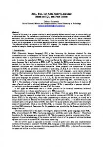
1.1 Historical overview of Annis A predecessor of the system – now called Annis 1 – was developed within the Sonderforschungsbereich 632 at the University of Potsdam [25]. It became apparent that Annis 1 was not particularly suited for large corpora because of its in-memory architecture and a desire to integrate the system with a database emerged. At the same time, the Humboldt-University of Berlin was developing a SQL compiler for DDDquery, the query language used by the DeutschDiachronDigital project [29, 2]. In an effort to reuse code, a simple mapping from the Annis 1 query language to DDDquery was devised, so Annis 1 could support a database back-end as fast as possible. The time spent during the database port was used to simplify the Annis query language and extend it with new features. The project was also joined by Karsten Hütter who developed a web frontend for a linguistic search engine including an advanced AJAX query builder as part of his diploma thesis [18]. Today his work, of which a screen shot is shown in Figure 1, is the most visible part of the Annis 2 system as the user interacts with it directly.
Figure 1: Screenshot of the Annis 2 web application with a result for the query example in section 3.
5
1.2 Goals and structure of this work The goals of this work are to formally define the concepts used within Annis 2, to develop an implementation of the Annis 2 Query Language (AQL2) on top of a relational database host (RDBMS) that can be used interactively with large corpora, to study optimization techniques, and to provide detailed performance measurements of the entire system. We first provide a formal definition of the corpus model used by Annis including a mapping to a SQL schema in section 2. Then, in section 3 we discuss the features of the Annis 2 Query Language including query functions. In section 4 we provide a reference implementation of AQL2 on top of the open-source RDBMS PostgreSQL. This section includes a detailed description on how graphs with multiple edge types can efficiently be supported on SQL hosts. We briefly discuss related work on evaluating XPath queries on relational databases and contrast Annis with TIGERSearch in section 5. The system is evaluated in section 6 for its performance on current consumer hardware on a moderately large corpus. Finally, in section 7 we summarize our findings and discuss on-going and future work on Annis. In the appendix we briefly discuss the Internal DDDquery implementation and provide an Annis 2 Query Language Grammar, the SQL Schema of the Corpus Data Model and a description of the Experimental Setup including information on the Tiger corpus.
6
2 Corpus Data Model 2.1 Overview The corpus data model defines a normalized representation of the information contained in an annotated corpus. It is used as an intermediary format to import the information generated by various annotation tools into the Annis service. During an import it is augmented with pre-computed, index-like information to implement different operations on the corpus data. Informally a corpus consists of one or more texts (primary data), such as a newspaper article, and annotations on these texts (secondary data). Individual text spans are modeled as nodes which are arranged in an ordered directed acyclic graph (ODAG). For each text an ordered subset of nodes define the tokens of the text. Edges between nodes can carry arbitrary semantic meaning. Currently we distinguish between edges that encode coverage, dominance and pointing relations between text spans. Nodes, edges and corpora can be annotated with key-value pairs. A corpus can also contain child corpora (called documents) which are arranged in a hierarchy.
2.2 Key concepts Definition 1 (Primary data) Any raw text can be used as primary data for a corpus. A primary data text has a unique identifier idtext and an informational name. Definition 2 (Text span) The triplet (idtext , left, right) defines a text span. It is the substring from left to right (inclusive) of the primary data text identified by idtext . Both left and right refer to character positions of the primary data text, starting with 0. Definition 3 (Token) Let t be a primary text and S a set of spans from t. A subset T ⊆ S is called the tokens of t if the following conditions hold: 1. T is well-ordered under a relation ≤pos , 2. ∀i, j ∈ T : i and $ let the user specify the relative position of two spans in a syntax tree. Annis 2 allows multiple syntax trees over the same spans. These are distinguished in the model using named edges and can be queried with >name or $name. By default Annis 2 will merge all syntax trees into 2 The
regular expression is evaluated by PostgreSQL which uses a POSIX-style syntax with a few extensions [24]. See the PostgreSQL manual, section 9.7.3. POSIX Regular Expressions.
12
Table 2: Possible coverage relationships between spans (not exhaustive). Span positions #1 _=_ #2 1: 2:
!
Coverage relation #1 _i_ #2
#1 _l_ #2
#1 _r_ #2
#1 _ol_ #2
#1 _or_ #2
#1 _o_ #2
!
!
!
!
! !
!
! ! !
!
! !
! ! ! ! ! ! !
1: 2: 1: 2: 1: 2: 1: 2:
!
1: 2: 1: 2:
a unified tree which is used in dominance operations if no name is given. Table 3 shows the different versions of > and $. Table 3: Dominance operations in AQL2. Operator
Definition
#i > #j
i directly dominates j (alias for #i >1 #j) i indirectly dominates j i dominates j with distance n i dominates j with distance n ≤ k ≤ m j is the left-most child of i j is the right-most child of i i and j share a parent i and j share an ancestor
#i #i #i #i #i
>* #j >n #j >n,m #j >@l #j >@r #j
#i $ #j #i $* #j
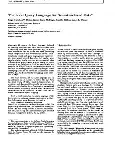
The direct dominance operators >, >@l, >@r and $ can optionally be qualified with a list of edge annotations enclosed in brackets [ and ], so that Annis 2 will only select dominance edges that are appropriately annotated. Like annotation search terms, the annotation key can be qualified with a namespace and the annotation value can be omitted or given as a regular expression. Figure 4 shows a syntax tree fragment demonstrating dominance between spans: • The upper cat="PP" span directly dominates the token span "zum" with a label func="AC" (#1 >[func="AC"] #3). • It also indirectly dominates the token "die" (#1 >* #4 and #1 >2 #4). • The token "Ukraine" is the right child of the lower cat="PP" span (#2 >@r #5). • "die" and "Ukraine" are directly dominated by the same node with a label func="NK" on both edges (#1 $ [func="NK"] #2). • Finally, "zum" and "Ukraine" share an ancestor span in the syntax tree (#3 $* #5). Dominance implies coverage, e.g. if #1 > #2 then #1 _i_ #2 and if #1 >@l #2 then #1 _l_ #2.
13
1:
cat = PP
AC
fun
fu
n fu 3:
...
cat = PP
2:
c=
=
c
=
NK
AC
func = NK
nc
NK
fun c=
fu
nc
4:
zum
1:0
für
=
NK
5:
die
Ukraine
...
Figure 4: Syntax tree fragment demonstrating different dominance relationships between spans. 3.3.3 Precedence The precedence operator . lets the user specify how many tokens two spans may be apart. Like coverage operations, precedence is only defined on spans of the same text. Table 4 shows the different versions of the precedence operator. Table 4: Precedence operations in AQL2. Operator
Definition
#i . #j #i .* #j #i .n #j
i i i i
#i .n,m #j
directly precedes j (alias for #i .1 #j) indirectly precedes j precedes j with distance n precedes j with distance n ≤ k ≤ m
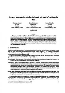
For token spans the precedence operator reflects their order in the annotation graph. Non-token spans are not ordered in the annotation graph per se, however the order of tokens induces an order on spans in an annotation graph. Definition 6 (Left-most, right-most covered token) Let s be a span. Then smin is the left-most and smax the right-most token covered by s. If we assume that the token order is described by a relation ≤pos , we can apply the precedence operator to non-token spans s and t by redefining ≤pos as s ≤pos t := smax ≤pos tmin . Figure 5 shows an annotation graph fragment demonstrating precedence between spans: • The token "zum" directly precedes the token "1:0" (#1 . #2). • "zum" also indirectly precedes the span annotated with cat="PP" (#1 .* #3 and #1 .2 #3). Note that the token "für" is the left-most child of cat="PP" in the embedded syntax tree. Because dominance implies coverage, "für" is therefore the left-most token covered by cat="PP". 3.3.4 Pointing relations The pointing relation operator -> allows queries for arbitrary links between two text spans. It follows the form of the dominance operator > except that the name is mandatory and that there is no support to query the left-most3 or right-most child. Table 5 shows the different variations of ->. 3 “Left
child” or “right child” would only make sense if there were a natural order on outgoing links.
14
cat=PP
3:
1:
...
2:
zum
1:0
für
die
Ukraine
...
token position
Figure 5: Annotation graph fragment demonstrating different precedence relationships between spans. Table 5: Pointing relation operations in AQL2. Operator
Definition
#i #i #i #i
i i i i
->name #j ->name * #j ->name n #j ->name n,m #j
directly points to j points to j, either directly or through intermediate nodes points to j with distance n points to j with distance n ≤ k ≤ m
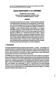
Like >, the direct pointing relation operator -> can be qualified with a list of edge annotations enclosed in brackets [ and ]. In Figure 6 pointing relations are used to encode the information structure of a text: • The red link relates the pronoun He to Sasha Muniak which occurred previously in the text. • The blue link indicates that the phrase Polish American further describes Sasha Muniak. IDENT
Its developer is a Polish American , Sasha Muniak . He had worked with . . . APPOS
Figure 6: Using pointing relations to model information structure.
3.3.5 Text span constraints There are a few unary linguistic constraints that only operate on one search term. They are listed in Table 6.
3.4 Combining expressions with OR The introductory example has already shown how search terms and linguistic constraints are combined with AND to build non-trivial queries. They can also be grouped with parentheses ( and ) and combined with | (logical OR) to build more complex expressions such as the following query: "the" & (("tree" & #1 . #2) | ("house" & #1 . #3))
This query could be stated in a more concise fashion using a regular expression search: "the" & /tree|house/ & #1 . #2
However, the longer version using OR is much faster; see section 6.7 for details.
15
Table 6: Unary linguistic constraints in AQL2. Operator
Definition
#i:root #i:arity = n #i:arity = m,n
i i i i i
#i:tokenarity = n #i:tokenarity = m,n
is a root node of an annotation graph has n children has m ≤ k ≤ n children covers n token covers m ≤ k ≤ m token
3.5 Meta data Given a query, Annis 2 generally searches all documents of a corpus, but the search can be confined to documents that have a specified meta annotation. The general form is meta::namespace:key="value" which looks like an annotation search term prepended with meta::. As with annotation search terms, the namespace and the value are optional and the value can be given as a regular expression. Note that although the syntax is similar, meta annotation definitions do not count as search terms and are skipped when evaluating search term references in linguistic expressions. They are also not considered when evaluating ORs. A document will only be searched if all meta annotations in the query are satisfied regardless of the alternative in which they appear.
3.6 Query evaluation Annis 2 evaluates queries in the following fashion: Let q be an AQL2 query and C a set of corpora on which q should be evaluated. First, if q contains meta annotation constraints they are stripped from q. Let D be the set of documents in C that satisfy every meta annotation constraint originally contained in q (or the set of all documents in C if q did not originally contain any meta annotation constraints). Then q is transformed into its disjunctive normal form q 0 = q1 ∨ . . . ∨ qn and each alternative is checked for validity. Definition 7 (Valid query) Let q be a query, qi an alternative of the disjunctive normal form of q and let qi contain k ≥ 2 search terms s1 , . . . , sk and l ≥ 1 binary linguistic constraints c1 , . . . , cl . Further, let #r be the reference to the r-th search term in qi , and let ⊗ be a placeholder for an arbitrary binary linguistic operator. Then qi is valid iff ∀si , sj :
(∃cp : cp is of the form #i ⊗ #j) ∨ ∃sr1 , . . . , srn , cr1 , . . . , crn+1 : cr1 is of the form #i ⊗ #r1 or #r1 ⊗ #i ∧ cr2 is of the form #r1 ⊗ #r2 or #r2 ⊗ #r1 ∧ ··· crn is of the form #rn−1 ⊗ #rn or #rn ⊗ #rn−1 ∧ crn+1 is of the form #rn ⊗ #j or #j ⊗ #rn
A query alternative consisting of exactly one search term and no linguistic constraints is always valid. The query q is valid iff all of its alternatives are valid. Informally, if we consider the search terms of an alternative as the nodes and the binary linguistic constraints as the (undirected) edges of a graph then the alternative is valid iff the corresponding graph is connected.4 4 This
requirement is necessary because the behavior of Annis 1, which implicitly assumes that unconnected groups of
16
Finally, for each alternative qi and each document d ∈ D Annis 2 will try to assign a span from d to each of the k span selection terms, so that each of the l linguistic constraints is satisfied. Definition 8 (Satisfied constraint, Solution) Let q be a query, q 0 its disjunctive normal form, and qi an alternative of q 0 with k search terms and l linguistic constraints c1 , . . . , cl and let cj be of the form #s ⊗ #t with 1 ≤ s, t ≤ k and ⊗ is a binary5 linguistic operator. Further, let d ∈ D be a document and T be a k-tuple of spans from d. We identify #s and #t with the s-th and t-th component of T respectively. Then T satisfies cj , iff the spans Ts and Tt are in the relationship described by ⊗. We call T a solution for qi , iff T satisfies every cj in qi . We call T a solution for q, iff there exists an alternative qi of q 0 for which T is a solution. Note that each alternative in q 0 may have a different number of span selections terms. Therefore, the size of a solution for q is not fixed, if its disjunctive normal form q 0 consists of more than one alternative. Annis 2 does not identify the alternative of which a tuple T is a solution but such identification is possible if the annotation graph fragment over T is retrieved. This process is described in the next section.
3.7 Query functions Knowing which spans are a solution to an Annis query is not all that interesting in itself. Researchers are typically interested in context or aggregate information. To this end, Annis 2 defines query functions that evaluate a query against a set of corpora and then retrieve additional information from the database based on the solutions to the query. Strictly speaking, query functions are not part of the Annis 2 query language. Instead, they encapsulate the steps that have to be taken to further analyze the solutions to a query after the solutions have been computed. Each query function corresponds to a analysis strategy supported by the Annis web interface. Before we can discuss query functions we have to define a few more concepts. Definition 9 (Preceding, following token) Let t be a token and let n ∈ N. Then t − n is the token preceding t by n tokens and t + n is the token following t by n tokens. Definition 10 (Annotation graph fragment) Let T be a set of primary data texts, A = (V, E) an annotation graph over T with nodes V and edges E and S a solution to a query from A in T . An annotation graph fragment over S with left context l and right context r is the subgraph of A consisting of the node set [ V0 = {v ∈ V : v overlaps a token from the interval [smin − l, smax + r]} s∈S
and the edge set E 0 = {(v, w) ∈ E : v, w ∈ V 0 } . Informally an annotation graph fragment contains all the tokens that are at most l tokens to the left or r tokens to the right of a span in a query solution, any span that overlaps these tokens, and all the edges in-between them. Definition 11 (Annotation matrix) Let A be an annotation graph, q an AQL2 query, S the set of solutions to q in A and let m be the maximum number of spans in a solution in S. The annotation matrix of S is a matrix that is constructed in the following fashion:
spans overlap, is very costly to implement. A query with n search terms and no linguistic constraint would require the addition of 2n alternative overlap constraints. The overlap operation is costly in itself (see section 6.1); to emulate the behavior of Annis 1 is thus prohibitive. 5 The process for unary operators is analogous: T satisfies an unary linguistic constraint of the form #s:⊗, iff the span Ts has the property described by ⊗.
17
1. For each tuple position 1 ≤ p ≤ m, the annotation keys6 Kp of any span Tp at position p in a solution T ∈ S are determined. [ Kp = {k : k is an annotation key of the p-th span in T } . T ∈S
2. The header of the matrix, i.e. the first row, is constructed by creating for each tuple (p, k) with k ∈ Kp .
Pm
p=1
kKp k cells, one cell
3. The body of the matrix, consisting of the following kSk rows, is constructed by creating a row for each solution T ∈ S. If the span Tp is annotated with a key k ∈ Kp then the corresponding cell contains the annotation value, otherwise it is empty. Currently Annis 2 defines the following three query functions. Let q be an AQL2 query, C a set of corpora on which q should be performed and S the set of solutions to q in C. • COU N T (q, C) returns the number of solutions in S. • AN N OT AT E (q, C, l, r) returns for each solution s ∈ S the annotation graph fragment over s with l tokens as left context and r tokens as right context. • M AT RIX(q, C) returns an annotation matrix for S in ARFF-Format [1].
3.8 Pagination of AN N OT AT E results The results returned by the AN N OT AT E query function can quickly become very large because it returns a complete annotation graph fragment for each tuple of spans matching the underlying query. Not only is the height of the annotation graph fragment unknown, but the width of the fragment can be arbitrarily extended by a user-defined context. Since the AN N OT AT E function is designed to be used interactively, returning the annotation graph fragments for every result is not sensible as the amount of the information presented would easily overwhelm the user. The frontend therefore enforces a pagination of the AN N OT AT E results similar to a web search engine: only the first n results of the query are displayed and the user can retrieve the next results if wanted. The number of results displayed on a page is user-configurable. Note that the Annis service supports the retrieval of all AN N OT AT E results at once; however, as section 6.6 shows, it is not optimized for this use case (the database handles this use case just fine).
3.9 Differences between ANNIS-QL 1 and AQL2 Although queries of the two languages look similar, there are quite a few differences: • A text search only covers tokens. There is currently no possibility to perform a real full text search in Annis 2. For example, in Annis 1 one can search for the phrase "the house"; in Annis 2 each token has to be specified separately and linked with the precedence operator: "the" & "house" & #1 . #2. • A text search has to match the entire text covered by a token. In Annis 1 a text search would implicitly match substrings as well. To match a substring in Annis 2 one can use a regular expression. • In Annis 1 one could search for spans by defining an annotation and the covered text in one expression (key=value:"text"). This syntax was very confusing in practice and is no longer allowed. The same search can be achieved with key="value" & "text" & #1 _=_ #2.
6 For
the purpose of this definition, the covered text of a span is considered an annotation of the span with the key
span.
18
• Annis 1 evaluates precedence in terms of the left and right text border of spans which results in nonintuitive behavior. For example, to search for an adjective followed by the string tree, one would have to write pos=ADJ & " tree" & #1 . #2. Note the space in " tree" which assumes that that all tokens in the text are separated by exactly one space. The Annis 2 corpus model makes the tokenisation that is present in the original data explicit and evaluates precedence in terms of the token position. Thus, in Annis 2 the query can be written as expected: pos="ADJ" and "tree" & #1 . #2. • There is no document search (doc=maz.*) in Annis 2. Using meta data to select documents is a much more powerful alternative. • Annis 1 implicitly assumes that text spans that are not used in any linguistic expression have to overlap. For example, pos=VVINF & cat=S would be converted to pos=VVINF & cat=S & #1 _o_ #2 before evaluation. In Annis 2, the first form is no longer possible because all search terms have to be connected to each other by a linguistic operation directly or indirectly. • Annis 1 interprets a single identifier as either a key or a value, e.g. pos would be expanded to pos=* | *=pos. Annis 2 treats single identifiers as an existence query, i.e. it selects any span annotated with the corresponding key, regardless of the annotation value. • Annotation type sets are not supported by Annis 2. • Annis 2 does not yet support NOT or XOR. • Annis 2 only allows normal parentheses ( and ) to group expressions. Brackets [ and ] are used to define edge labels.
19
4 SQL Generation In this section we will describe how an AQL2 query is translated into a SQL query. For historical reasons an Annis query is not translated directly to SQL, but translated to an intermediate DDDquery [29] first. The mapping from AQL2 language features to DDDquery language features is described in appendix B. Since it is almost trivial in nature, the rest of this section skips this intermediary step and assumes that the Annis query is translated directly to SQL. The translation from AQL2 to DDDquery is briefly described in appendix B. We will first demonstrate how to build a SQL query that generates all the solutions for a given Annis query from a list of corpora. Then, we will extend this general framework to include query functions as described in section 3.7.
4.1 Computation of derived node data during corpus import The evaluation of some operations requires information that is not explicitly present in the corpus schema and which first has to be derived from other data contained therein. This information is fixed for each node; it is therefore advisable to perform the computation only once during corpus import and cache the results in the node and rank tables. However, each additional column will generally slow down the evaluation of queries because for each node PostgreSQL has to load more data from disk. A trade-off has then to be found between improving the performance of a specific operation and the general performance on typical queries. For example, we have decided against caching the node arity described in section 4.3.9 because we have not seen it used in actual queries. 4.1.1 Minimally and maximally covered tokens In section 3.3.3 we extended the token order relation ≤pos to non-token spans s and t by comparing the right-most and left-most covered token smax and tmin : s ≤pos t := smax ≤pos tmin During import we set tmin := tmax := t for each token span t and compute smin and smax for each non-token span s. We then extend the node table with the attributes left_token and right_token which for each span s store the value of node.token_index of smin and smax respectively. 4.1.2 Root nodes in the original ODAG In section 4.3.7.2 we describe how the original ODAG is partitioned to implement the dominance and pointing relationship operators. This can create partitions rooted in a node that is a leaf in another partition; in other words it creates many false roots. A true root in the original ODAG will be a root node in any partition it appears in. The following SQL query finds all such nodes: SELECT node_ref FROM rank GROUP BY node_ref HAVING count(DISTINCT rank.parent) = 0;
During import we extend the rank table with the attribute root and set it to TRUE if the corresponding node is selected by the above query and to FALSE if it is not.
20
4.1.3 Identification of a node’s top-level corpus The corpus schema defined in section 2.3 links each node with the document that contains the corresponding text span. If a search is restricted to a document d, all documents below d have to searched as well; in section 4.5 we describe a general way to achieve just this. However, the Annis frontend only exposes top-level corpora and each top-level corpus is imported individually. It is therefore easier and faster to extend the node table with an attribute toplevel_corpus which is a foreign key to corpus.name and store in it the name of top-level corpus being imported.
4.2 The SELECT and FROM clauses Internally, a span is identified by the primary key of its node in the database database, node.id. This attribute is (mostly) meaningless to the Annis frontend but the SELECT clause is highly dependent on the query function used, and right now we are only interested in generating solutions for a given query. Consider a query without disjunctions, containing n search terms. For this query we access the node table via n aliases in the FROM clause and select their id attributes in the SELECT clause. This strategy generates one row in the result set for each solution to the query. We use the DISTINCT keyword to ensure set semantics. SELECT DISTINCT node1.id, node2.id, ..., nodeN.id FROM node AS node1, node AS node2, ..., node AS nodeN ...
Recall that the tuple length is not necessarily the same for each solution if the query contains more than one alternative. However, in the SQL fragment above we have fixed the number of columns and accessed table aliases. We will defer the resolution of this conflict to section 4.4 and assume for the rest of this section that the Annis query consists of only one alternative, unless otherwise noted. The SELECT clause is now complete. The FROM clause on the other hand only reference the node table which contains the necessary information to implement a node or text search and the precedence and coverage operators. If the query contains an annotation search or any other linguistic constraint, the tables node_annotation, rank, component and edge_annotation are needed. If a query requires information from another table to implement an operation involving a search term, the compiler will create a table alias for this table and join it to the corresponding node table alias. It is sufficient to join each table only once to the node alias except for the edge_annotation table. The direct dominance and pointing relation operators can be qualified with multiple edge labels and the compiler has to create one edge_annotation table alias for every label. Listing 1 shows the FROM clause that is generated for the query example in section 3.1.
4.3 The WHERE clause: Translation of AQL2 language features In this section we will show how AQL2 language features translate to conditions in the WHERE clause. For search terms and unary linguistic constraints we will assume that the appropriate tables are accessed via an alias with index 1 in the FROM clause. For binary constraints we assume the existence of table aliases with index 1 for the left-hand-side span and index 2 for the right-hand-side span. 4.3.1 Text search A text search "Mary" or tok="Mary" is realized by comparing the text with the attribute node1.span.
21
Listing 1: FROM clause generated for the Annis query example in section 3.1. FROM node AS node1 JOIN node_annotation AS node_annotation1 ON (node_annotation1.node_ref = node1.id) JOIN rank AS rank1 ON (rank1.node_ref = node1.id) JOIN component AS component1 ON (rank1.component_ref = component1.id), node AS node2 JOIN rank AS rank2 ON (rank2.node_ref = node2.id) JOIN component AS component2 ON (rank2.component_ref = component2.id) JOIN edge_annotation AS edge_annotation2_1 ON (edge_annotation2_1.rank_ref = rank2.pre), node AS node3 JOIN node_annotation AS node_annotation3 ON (node_annotation3.node_ref = node3.id) JOIN rank AS rank3 ON (rank3.node_ref = node3.id) JOIN component AS component3 ON (rank3.component_ref = component3.id), node AS node4 JOIN rank AS rank4 ON (rank4.node_ref = node4.id) JOIN component AS component4 ON (rank4.component_ref = component4.id) JOIN edge_annotation AS edge_annotation4_1 ON (edge_annotation4_1.rank_ref = rank4.pre)
node1.span = ’Mary’
Note that the span attribute contains the content of a text span for tokens only and is set to NULL for non-tokens. This corresponds to the property of the text search that it can only be used for token spans. To implement a text search with a regular expression like /Mar(y|ie)/ we use the PostgreSQL-specific operator ~ which matches its left-hand side to a regular expression on the right-hand side. node1.span ~ ’^Mar(y|ie)$’
Note that the regular expression is always explicitly anchored as required by the definition of the regular expression text search in AQL2. 4.3.2 Token search To search for any token we simply select those tuples from the node table where the attribute span is not set to NULL: node1.span IS NOT NULL
Alternatively, we can use the token_index attribute which is also set to NULL for any non-token span: node1.token_index IS NOT NULL
4.3.3 Annotation search To implement an annotation search we compare the components of the search term to the attributes namespace, name and value of the node_annotation table. For example, a search for a span annotated with tiger:cat="S" is realized by the following conditions: node_annotation1.namespace = ’tiger’ AND node_annotation1.name = ’cat’ AND node_annotation1.value = ’S’
22
An annotation search with a regular expression is implemented in the same manner as a regular expression text search; the regular expression is explicitly anchored and matched using the PostgreSQL pattern matching operator ~ (tilde). If an optional part of an annotation search is missing then the constraint on the corresponding table attribute is omitted as well. 4.3.4 Node search The search term node places no constraint on the spans selected from the annotation graph. Accordingly, it requires no conditions in the WHERE clause. Simply listing an alias to the node table in the FROM clause is enough to implement a node search. 4.3.5 Coverage Coverage operations are defined as a comparison of the left and right borders of two spans of the same text. The span borders are stored in the attributes node.left and node.right and the text is referenced by the foreign key node.text_ref. To implement a coverage operator, we substitute each span property in the operator definitions in Table 1 in section 3.3.1 with the corresponding table attribute of the node table (see section 2.3). For example, the exact-cover constraint #i _=_ #j is realized by the following conditions: node1.text_ref = node2.text_ref AND node1.left = node2.left AND node1.right = node2.right
4.3.6 Precedence In Annis 2, precedence is defined in terms of tokens. The term #i . #j conveys that there should be no token between the spans i and j, regardless of any possible whitespace that may exist between them in the original primary text.7 Similarly, the term #i .n #j conveys that i and j should be exactly n tokens apart (which is not possible to express in Annis 1 at all). In section 3.3.3 we have shown how the token order relation ≤pos is extended to non-token spans s and t by comparing the right-most and left-most covered token smax and tmin : s ≤pos t := smax ≤pos tmin
(1)
We can use Equation 1 to formally define the variants of the precedence operator listed in Table 4: #i . #j #i .* #j #i .n #j #i .n,m #j
⇐⇒ ⇐⇒ ⇐⇒ ⇐⇒
imax = jmin − 1 i jpost ipre < jpre < ipost
(3)
The last transformation in Equation 3 is motivated by the usage of one counter for both pre-order and post-order. If we substitute the corresponding table attributes we arrive at: rank1.pre < rank2.pre AND rank2.pre < rank1.post
Of course, for direct dominance we can exploit the attribute rank.parent which is conveniently provided by the Annis converter: rank1.pre = rank2.parent 8 Dominance
edges called edge and secedge are artifacts of a TIGERSearch-annotated corpus.
24
4.3.7.2 Separation of dominance and pointing relation edges in the annotation graph However, the definition of the dominance relation in Equation 3 is incomplete, since it tests for the existence of any path between two spans and disregards the semantic meaning of the edges along that path. For example, in Figure 7 the span g does not dominate d0 because the edge between g and d0 encodes a pointing relation. Even if the first and the last edge of a path are dominance edges, there might still be a pointing relation edge somewhere in the middle such as in the path from e to c00 . It is therefore necessary to restrict Equation 3 in such a way that all edges along a path between two spans are of the same type. To this end, we partition the annotation graph into connected components such that each edge in a particular component is of the same type. The implementation of the dominance relation can then be completed by checking the edge type of the first (or last) edge and making sure that there is a component that contains both spans. This can be expressed with the following conditions: component1.type = ’d’ AND component1.id = component2.id
The Annis converter computes the pre- and post-order values in such a way that Equation 3 holds, iff there exists a component with both spans. The last condition can thus be omitted. Figure 8 shows the components of the annotation graph in Figure 7. As expected there is no component of dominance edges that contains a path from g to d0 or from e to c00 . If the original annotation graph contains nodes that are connected to two or more parent nodes by different edge types (e.g. the span d), then the partitioning strategy will create components that are completely contained in another component in the partitioned graph (e.g. component (c) is contained in (a) in Figure 8). These are pruned from the database by the Annis converter to save space. (a)
(b) 1
2
3
c
4
b
a
16
se ce dg e
9
5
6
10
d
c0
8
11
f
17
20
d0
IDENT
e
15
18
g 12
(c)
g
13
7
14
d0
19
c00
x
x
x
x
Figure 8: Annotation graph partitioned by edge type. The components (a) and (c) contain only dominance edges while (b) contains only pointing relation edges. Component (c) is pruned from the database. Edges in Annis have a second property that conveys semantic meaning, their name. While named edges are rarely used in dominance relations, they are mandatory for pointing relations: the term #i ->IDENT * #j requires that all edges on the path from i to j have the name IDENT. Conceptionally, a name is nothing but a subtype. To ensure that all edges along a path have the same name, we partition the graph along the distinct combinations of edge type and name. Figure 9 shows the generated components for the annotation graph in Figure 7. We can now ensure that every edge along a path has a certain name, by checking the name of the first (or last) edge: component1.name = ’IDENT’
25
(a)
(b) 1
a
10
(c) 11
a
(d)
14
15
e
20
21
secedge
2
3
c
4
b
9
5
6
12
d
c0
(e)
g 24
d0
IDENT
e
13
16
g
f
17
18
8
7
19
22
d0
23
c00
x
x
x
x
Figure 9: Annotation graph partitioned by edge type and name. Component (e) is pruned from the database because it is contained in component (a). 4.3.7.3 The unnamed dominance operator variant Annis 2 will merge all syntax trees of a given graph into one unified tree that is searched if the dominance operator is used without a name. Consequently, the term #i >* #j only requires that edges on a path from i to j are dominance edges. Their name is not only irrelevant but each edge can have a different name as in the path from a to g in Figure 7. Unfortunately, when we partitioned the annotation graph along edge names, we only retained paths where each edge has the same name. The solution is to take the dominance components of the type-partitioned graph, set their name to NULL and test for a path in any of these components. Figure 10 shows all the components that are created for the annotation graph in Figure 7. 4.3.7.4 Length-restricted dominance operator variants To implement the length-restricted variants of the dominance operator >n and >n,m, we need to be able to measure the length of a path between two nodes. We can achieve this by computing the depth of each node and only return those nodes i and j which are connected by a path of length n = jdepth − idepth .
(4)
At first glance, this approach poses three problems: 1. The depth of a node is defined as the distance from the root to the node. An annotation graph can have multiple roots; which one should we choose? 2. For any two nodes i and j there may be multiple paths between i and j in the annotation graph, each with a different length. 3. The partitioning described in section 4.3.7.2 can introduce many false roots, such as the node e in Figure 10. As a consequence, the computation of the node depth will yield different results depending on whether it is done before or after graph partitioning. The first issue disappears once we have assigned pre- and post-order values to the nodes. If the original annotation graph had multiple roots, the pre/post-order traversal generates a forest of trees and we can compute the node depth for each tree individually. The second issue is actually a feature of Annis. For example, we want to find the spans b and c as solutions for the term #i > #j as well as #i >1 #j. This is possible because the pre/post-order traversal effectively creates a copy of c to which we can assign a different depth.
26
(a)
(b) 1
a
16
17
a
26
edge
b
9
10
e
15
18
b
edg
c
4
5
d
8
11
g
f
12
13
14
19
c
20
e
3
25
edg
e
2
21
d
24
edge
6
c0
7
(c)
(d)
edg
32
(e) 33
30
31
34
(f)
g 36
secedge
g 29
a
37
40
35
38
d0
23
(g) 0
d0
c00
c00
d
IDENT
e
c0
edge
f
e
e edg
e
27
28
22
39
Figure 10: Annotation graph components for each edge type and name and the merged syntax tree. Components (a) and (f) contain the merged syntax tree, components (b), (c) and (g) contain dominance edges called edge, component (d) contains a secedge dominance edge and component (e) an IDENT pointing relation. Components (f) and (g) are pruned from the database because they are contained in (a) and (b) respectively. Finally, the exact values for the node depth are irrelevant, since we’re only interested in the distance between nodes. It follows from these considerations that the depth of a node has to be stored in the rank table. During import we extend the rank table with the attribute depth in which we store the depth for each node. Substituting this attribute into Equation 4 we arrive at the following condition for the term #i >n #j: rank1.depth = rank2.depth - n
The term #i >n,m #j is implemented in a similar fashion: rank1.depth BETWEEN SYMMETRIC rank2.depth - n AND rank2.depth - m
4.3.7.5 Left-most and right-most dominance operator variants To implement the dominance operators >@l and >@r we exploit the fact that the computation of the preand post-order values follows the order of the children of a node. In other words, for each non-terminal i and its left-most child l and right-most child r the following conditions hold: ipre ipost
= =
lpre − 1 rpost + 1
(5)
In the original unpartitioned annotation graph the left-most (or right-most) child identified by Equation 5 could potentionally be connected to the parent node by a pointing relation edge. However, once the
27
annotation graph is partitioned along edge types, there can be no pointing relation edge in a dominance component. Substituting the corresponding table attributes into Equation 5 we arrive at the following condition for >@l: rank1.pre = rank2.pre - 1 >@r
is implemented in a similar fashion: rank1.post = rank2.post + 1
4.3.7.6 Same parent and same ancestor dominance operator variants The implementation of the dominance operator $ is simple as we explicitly store a pointer to the parent of a node in the attribute rank.parent. Thus, two nodes share a parent if there exists a dominance component for which the corresponding entries in the rank table have the same value in parent: rank1.parent = rank2.parent
If two nodes s and t share a common ancestor c then the following Equation 6 must hold for both c and s and c and t: s and t share an ancestor ⇐⇒ =⇒
∃ node c : cpre < spre < cpost ∧ cpre < tpre < cpost s, t and c are connected
(6)
We can express this relationship using a subquery in an EXISTS clause: component1.id = component2.id AND EXISTS ( SELECT 1 FROM rank AS ancestor WHERE ancestor.component_ref = component1.id AND ancestor.pre < rank1.pre AND rank1.pre < ancestor.post AND ancestor.pre < rank2.pre AND rank2.pre < ancestor.post )
4.3.7.7 Edge annotations Dominance and pointing relation operations between parent and child spans (i.e. >, >@l, >@r, $ and ->) may be qualified with a list of edge annotations to search for particular edges. The test for an edge annotation is similar to a node annotation search using the edge_annotation table which contains a foreign-key to the rank table. Because each tuple in rank is interpreted as an incoming edge, we have to use the edge_annotation table alias created for the right-hand-side of the operator which is expressed by the index 2 before the underscore. edge_annotation2_1.namespace = ’tiger’ AND edge_annotation2_1.name = ’func’ AND edge_annotation2_1.value = ’OA’
Recall that we can qualify the dominance and pointing relation operator with multiple edge annotations. We need to access a different edge_annotation table alias for each listed annotation. In the example above we have assumed that we are looking for the first annotation in the list, denoted by the index 1 after the underscore. The same parent operator $ is an exception to the rule that we have to test the right-hand-side of the operator. For $ we want to make sure that both nodes are connected to a parent by accordingly annotated edges. We thus need to test the edge_annotation aliases created for both nodes.
28
4.3.8 Root nodes In the original unpartitioned annotation graph a root node is identified by its parent attribute being set to NULL. Unfortunately, the partitioning of the annotation graph described in section 4.3.7.2 may introduce many false roots, i.e. nodes which are a root node in one component and a leaf node in another component. For example, in Figure 10 the node e is the root of component (c) and a leaf in component (d). To correctly implement the root operator #i:root, we must only consider nodes as roots which are a root node in all components in which they appear. These are identified by the attribute root of the rank table which is computed during corpus import. The term #i:root can thus be implemented by testing the root attribute: rank1.root IS TRUE
4.3.9 Node arity The node arity, i.e. the number of children for a given node v, can be determined by counting the entries in the rank table which point to v via the parent attribute. The term #i:arity=n can thus be implemented as follows: (SELECT count(DISTINCT children.pre) FROM rank AS children WHERE children.parent = rank1.pre) = n
The term #i:arity=n,m is implemented in a similar fashion: (SELECT count(DISTINCT children.pre) FROM rank AS children WHERE children.parent = rank1.pre) BETWEEN SYMMETRIC n AND m
We have left out the restriction on a particular component in the SQL fragments above because we assume that it is selected by another linguistic constraint in the Annis query. 4.3.10 Token arity During corpus import we have identified the left-most and right-most covered token of a given span s and stored their index in the attributes node.left_token and node.right_token respectively. We can use these attributes to implement the token arity operator: s covers n token
⇐⇒
n = smax − smin + 1
(7)
Transforming Equation 7 and substituting the corresponding table attributes, we arrive at the following conditions for the term #i:tokenarity=n: node1.text_ref = node2.text_ref AND node1.left_token = node2.right_token - n + 1
Similarly, the term #i:tokenarity=n,m can be translated as follows: node1.text_ref = node2.text_ref AND node1.left_token BETWEEN SYMMETRIC node2.right_token - n + 1 AND node2.right_token - m + 1
This concludes the SQL generation for a query with only one alternative. In the next section, we will see how to transform queries that contain multiple query alternatives into SQL code.
29
4.4 Query alternatives During the discussion of the SELECT and FROM clauses we have already alluded to an apparent shortcoming of the strategy to model a query solution as a tuple of node.id attributes: whereas the solutions to a query with multiple alternatives may vary in size, the tuple size returned by a SELECT statement is necessarily fixed. Suppose that we have a query q consisting of two alternatives q1 containing n search terms and q2 containing m search terms and n < m. We will then need at least m aliases for the node table and any other table that may be required to solve the alternative q2 . Suppose further that we use the first n table aliases for both alternatives and construct the query for q in the following fashion: SELECT DISTINCT node1.id, node2.id, ..., nodeM.id FROM node AS node1 JOIN ..., node AS node2 JOIN ..., ..., node AS nodeM JOIN ... WHERE ( (
conditions for q1 ) OR conditions for q2 )
This strategy causes two interrelated problems: 1. Let’s assume that we need to join an annotation table to the node table representing the span at position p in the solutions for q1 . Let’s assume further, that there exists no tuple in this annotation table that could be joined against the nodes selected at position p for q2 .9 Because of the semantics of JOIN, an empty set will be selected for the candidates at position p which in turn will produce an empty result for the entire alternative q2 . 2. Because the conditions generated for q1 place no constraint on the table aliases with an index bigger than n, the solutions returned for q1 will consist of the cartesian product of the actual solutions and any span in the database for the tuple positions n + 1 ≤ p ≤ m. The first issue can be mitigated against by using a LEFT OUTER JOIN for annotation tables. However, solving the second problem requires a case differentiation in the SELECT clause using CASE ... WHEN ... THEN statements which quickly gets very complicated the more alternatives a query has. A much simpler solution is to pad the SELECT clause of q1 with NULL values and append the results for q1 and q2 using UNION as shown in Listing 2.
4.5 Corpus selection Until now we always searched the entire database when looking for solutions to a query. This is fine for single-user systems but Annis was designed with many users in mind and the frontend only exposes those corpora which a particular user is allowed to use. We thus need a way to filter for (top-level) corpora which are referenced by the query (generated from the frontend) by their (unique) names. If a query is to be performed against a document d then every document below d in the corpus hierarchy has to be searched as well. The node table is connected to the corpus table via the corpus_ref foreign key. To restrict the search to a particular document called name and all its children, we can use the following condition for each node table alias i used in the query: nodei.corpus_ref IN (SELECT child.id FROM corpus AS child, corpus AS doc WHERE child.pre BETWEEN doc.pre AND doc.post AND doc.name = ’name’) 9 This
case is arguably rare for node_annotation but it happens quite often for edge_annotation.
30
Listing 2: SQL query template for Annis queries with multiple alternatives using UNION. SELECT DISTINCT node1.id, node2.id, ..., nodeN.id, NULL, ..., NULL {z } | FROM m − n times node AS node1 JOIN ..., node AS node2 JOIN ..., ..., node AS nodeN JOIN ... WHERE
conditions for q1 UNION SELECT DISTINCT node1.id, node2.id, ..., nodeM.id FROM node AS node1 JOIN ..., node AS node2 JOIN ..., ..., node AS nodeM JOIN ... WHERE
conditions for q2
However, the frontend only exposes top-level corpora. During corpus import we have extended the node table with an attribute toplevel_corpus which links each node v to the top-level corpus of the document containing v. We can therefore implement the selection of corpora with a constraint on this attribute. To enhance readability, we create a view of the node table containing only the nodes of the requested corpus name and refer to this view instead of the node table in the query. We need to wrap the creation of the view and the execution of the query inside a transaction so that multiple queries against the database can be run concurrently without manually managing view names: BEGIN; CREATE VIEW node_v AS SELECT * FROM node WHERE node.toplevel_corpus = ’name’; SELECT node1.id, ... FROM node_v AS node1 ... ... ROLLBACK;
4.6 Meta data filtering For queries containing a meta data specification we only want to search documents below the requested root document that are properly annotated. We can piggy-back this condition on the view created in section 4.5. For example, the term meta::lang:l1="de" creates the following view: CREATE VIEW node_v AS SELECT * FROM node JOIN corpus_annotation AS corpus_annotation1 ON (node.corpus_ref = corpus_annotation1.corpus_ref) WHERE node.toplevel_corpus = ’name’ AND corpus_annotation1.namespace = ’lang’ AND corpus_annotation1.name = ’l1’ AND corpus_annotation1.value = ’de’;
31
If the Annis query contains multiple meta data annotations, we have to join a separate corpus_annotation table alias to the node table for every listed annotation. The SQL generation for an Annis query is now complete. In the next section we will describe how the query functions defined in section 3.7 are implemented.
4.7 Query functions 4.7.1 The COU N T function The COU N T function is implemented by wrapping the original query as a subquery and counting the solutions using count(*) in the outer query. 4.7.2 The AN N OT AT E function The AN N OT AT E function can be implemented by using the SQL query generated for an Annis query q as a subquery to generate the solutions S to q and then retrieve the overlapping tokens of the annotation graph fragment over S in the outer query. For this to work we need to modify the SELECT clause of the inner query to return the attributes needed to implement the overlapping operator: SELECT DISTINCT node1.id AS id1, node1.text_ref AS text1, node1.left_token node2.id AS id2, node2.text_ref AS text2, node2.left_token ..., nodeN.id AS idN, nodeN.text_ref AS textN, nodeN.left_token -
lef t AS min1, node1.right_token + right AS max1, lef t AS min2, node2.right_token + right AS max2,
lef t AS minN, nodeN.right_token + right AS maxN
In the SQL fragment above, lef t and right specify how much context the annotation graph fragment returned by AN N OT AT E should contain. The outer query is depicted in Listing 3. Three features are worth mentioning: 1. The attributes node.id of the spans in a query solution are concatenated to create a key which groups all the spans of a retrieved annotation graph fragment (line 2). 2. We use OFFSET and LIMIT to retrieve only the annotation graph fragments for a subset of the query solutions to enable the pagination feature of the frontend described in section 3.8 (line 7). This requires that the result returned by the inner query is sorted which is achieved by the ORDER BY clause. 3. The result of the outer query is ordered by the key identifying an annotation graph fragment and the pre-order value to ease the reconstruction of the annotation graph in the application (line 24). The result set returned by this query can be transformed into an annotation graph using an algorithm that is similar to the gXDF reconstruction of a DDDquery result described in [28]. A simple walk through the result set represents a pre-order traversal of the graph we want to reconstruct. We keep track of the nodes and edges we have already seen as well as their annotations to skip through the result set if possible. Once we encounter a new key, we know that the current annotation graph fragment is complete and start a new one. 4.7.3 The M AT RIX function To implement the M AT RIX function, we need to modify the SELECT clause to retrieve the node annotations belonging to a span. If we simply retrieved the attributes of the node_annotation table for
32
Listing 3: SQL query used by the AN N OT AT E function to retrieve the annotation graph fragments over the solutions to a query q. 1 2 3 4 5 6 7 8 9 10 11 12 13 14 15 16 17 18 19 20 21 22 23 24
SELECT DISTINCT (matches.id1 || ’,’ || ... || ’,’ || matches.idN) AS key, facts.* FROM (
SQL query generated for q with modified SELECT clause ORDER BY id1, ..., idN OFFSET of f set LIMIT limit ) AS matches, ( node JOIN rank ON (rank.node_ref = node.id) JOIN component ON (rank.component_ref = component.id) JOIN node_annotation ON (node_annotation.node_ref = node.id) JOIN edge_annotation ON (edge_annotation.rank_ref = rank.pre) ) AS facts WHERE ( facts.text_ref = facts.left_token ) OR ... OR ( facts.text_ref = facts.left_token )
matches.text1 AND = solutions.min1 matches.textN AND = solutions.minN
ORDER BY key, facts.pre
each span, the result set would quickly grow very large. For example, if a query q contains n search terms and each span has m annotations, we would need mn rows in the result set for one solution alone. Furthermore, the set semantics of the original SQL query, i.e. one row representing one solution to q, would be lost complicating the application code that has to parse the result set. A solution to this problem is to aggregate the annotations for one span into an array using the PostgreSQL-specific aggregate function array_agg: SELECT node1.id AS id1, substr(text1.text, node1.left, node1.right - node1.left + 1) AS span1, array_agg(DISTINCT coalesce(node_annotation1.namespace || ’:’, ’’) || node_annotation1.name || ’=’ || node_annotation1.value), ... nodeN.id AS idN, substr(textN.text, nodeN.left, nodeN.right - nodeN.left + 1) AS spanN, array_agg(DISTINCT coalesce(node_annotationN.namespace || ’:’, ’’) || node_annotationN.name || ’=’ || node_annotationN.value) ... GROUP BY id1, span1, ..., idN, spanN
We also retrieve the covered text for each span in accordance to the definition of the M AT RIX function. The coalesce function is used to ensure correct results in case the namespace attribute is set to NULL. The result set of this query can be transformed into an annotation matrix using the algorithm described in definition 11.
33
5 Related work As we have mentioned in section 3, the Annis query language is influenced by NiteQl and TIGERSearch. The NITE XML Toolkit uses Apache Xerces as its XML-processing backend [9, 3], but TIGERSearch is implemented as a custom application written in Java. In this section, we will briefly compare TIGERSearch to Annis. Because Annis queries are first translated to DDDquery, which is based on XPath, we will also briefly discuss the research on evaluating XPath queries on relational database hosts.
5.1 TIGERSearch The TIGERSearch query language was developed as part of the TIGER Treebank, a corpus of 40000 syntactically annotated sentences from German newspapers [8]. Similarly to Annis, it models sentences as two-dimensional trees: the syntax structure of a sentence is encoded by parent-child relationships of nodes and the word order is encoded by explicitly ordering the tree’s leaves. Additionally, the TIGER data model allows for secondary edges between nodes if the syntax structure cannot be adequately captured by a tree. A major difference to Annis is that each text span is represented by exactly one node. This is most obvious when multiple attributes of a span are queried at once. For example, the following Annis query looks for the possessive form of the German article die: "der" & morph="Gen.Sg.Fem" & #1 _=_ #2. Using TIGERSearch, this query can be shortened to: [word="der" & morph="Gen.Sg.Fem"]. TIGERSearch has no need for coverage operations because it works on unambiguously annotated corpora, whereas Annis supports corpora with conflicting annotations. As with Annis, nodes are assembled into a graph template using dominance and precedence relations and constraints such as node arity. TIGERSearch supports negation for attribute values and node relations. Originally, it did not support universal quantification for negated values, but this was added as part of the Stockholm TreeAligner, a search tool for parallel treebanks based on TIGERSearch [22, 30]. An interesting feature of TIGERSearch is that a subset of the query language is also used as the corpus description language for the TIGER Treebank. This design strongly influences the implementation of the query processor. It is based on logical programming languages, specifically on the resolution of Horn clauses: given a graph g and a query q, TIGERSearch tests if it can find a set of nodes so that g ∪ q is contradiction-free [21]. Before a corpus can be searched it must be preprocessed. This generates the index – a proprietary, domain-specific column store. Each attribute value is stored in an attribute-specific list which is indexed by the node id. Furthermore, attribute values are dictionary-encoded to reduce space. The index also contains lists for other node properties, such as node arity and continuity and the node id of the left-most and right-most leaf to allow a quick implementation of left-most and right-most dominance as well as precedence. Finally, it contains the Gorn address of each node to quickly test for node dominance: a node s dominates another node t if the Gorn address of s is a real prefix of the Gorn address of t [13]. This index is conceptionally similar to the materialized facts table introduced in section 6.3. The discussion of the index data structure shows that the implementation of the precedence operator is almost identical to Annis. The only difference is that TIGERSearch reduces precedence of non-terminal nodes to the left-most leaves whereas Annis takes both the left-most and the right-most leaves into account. The dominance operator is implemented differently in TIGERSearch and Annis, but both concepts are just as expressive. Gorn addressing, originally developed to encode a tree structure can be adapted to ODAGs in the same way as pre/post-order addressing was adapted for DDDquery: A node which can be reached by more than one path from a root will have multiple Gorn addresses. During the preprocessing phase of a corpus, TIGERSearch also generates statistics about the selectivity of each attribute value by building an inverted list, pointing from an attribute value to the containing graphs, for values below a configurable frequency.10 Then, before evaluating a query, it first determines 10 In
the TIGER Treebank, a corpus normally consists of multiple graphs, each representing a sentence.
34
the most restrictive query term and the graphs that are a match for this term. The evaluation of the entire query is then limited to those graphs.
5.2 Evaluating XPath queries using relational databases In recent years there has been a wealth of research regarding the efficient evaluation of XPath queries on SQL hosts. Two different approaches can be identified: schema-based systems which use information derived from a DTD or XML Schema definition to create a relational representation of the data stored in XML documents and schema-oblivious systems which strive to find a relational representation of XML documents independent of any particular schema [20]. The pre/post-order scheme proposed for DDDquery [28] was originally developed as part of the XPath Accelerator [15] and is an example of a schema-oblivious system. This is a good match to the requirement of Annis to store conflicting annotation graphs from multiple annotation tools without a predefined tag set. The key observation of the XPath Accelerator is that the pre- and post-order values of a node in a XML tree partition the pre/post-plane of the document in four non-overlapping regions which directly correspond to the major XPath axes ancestor, descendant, preceding and following. DDDquery retains the ancestor and descendant axes but redefines the preceding and following axes to refer to the position of a span in a linear text and not its position in a tree and/or graph over tokens from that text. A number of index structures and join algorithms have been proposed to efficiently evaluate XPath location steps along the ancestor and descendant axes, such as the use of Patricia keys to encode root-toleaf paths [11] or the Structural Join (also called Containment Query) to quickly find ancestor-descendant relationships between two ordered lists of candidate nodes [31, 5, 10]. Unfortunately, most of these schemes require changes to the underlying database kernel and thus were not feasible as part of the Annis project. Of particular interest is the Staircase Join algorithm [17]. An implementation11 exists for PostgreSQL and many of its ideas can be expressed in purely relational terms [23, 16]. As it turns out, however, it achieves its remarkable performance by exploiting the semi-join semantics of XPath. To compute the result of a XPath location step starting from a set of context nodes C, not all nodes in C have to be evaluated. Those that contribute no new nodes because their target nodes are contained in the target nodes of another node in C can be pruned. The same is not true in a DDDquery expression. Here we are not only interested in the target nodes of the last location step but potentially in any nodes that were found along the entire DDDquery path expression. Nevertheless, some of the ideas in [16] can be adapted for Annis, namely the use of partitioned B-Trees to narrow down candidate nodes while computing joins. Fortunately, the mapping from Annis to DDDquery uses the descendant axis almost exclusively to define operators that refer to a span’s position in a graph. Using a combined pre/post-order scheme, a step down the descendant axis can be computed using a bounded range lookup on a single value which is efficiently supported by B-Trees. The only operator that maps to the ancestor axis is the common-ancestor operator which benefits from an early-out strategy and is further sped up by the explicit partitioning of the graph into connected components. The MonetDB/XQuery processor was also adapted to linguistic corpora based on multiple stand-off XML documents much like PAULA [7, 6]. It can query documents larger than 1GB interactively but a direct comparison with Annis is difficult because of differences in the underlying XML structure.
11 The implementation is for PostgreSQL 7.4 which has been outdated for quite a while now. This reflects the ongoing effort by the developers to implement efficient XPath processors on off-the-shelf SQL databases. A loop-lifted variant of the Staircase Join is used in MonetDB/XQuery.
35
6 Evaluation and Optimization The goal of this section is to analyze the performance of Annis 2 and improve it to a point where the system can be used interactively. Specifically, we want to achieve an evaluation time of less than two seconds for typical queries on a large corpus on current consumer hardware. We used the 12 test queries listed in Table 23 on page 62 which were provided by users of the Annis system. The queries were evaluated against the Tiger corpus, a fairly large and deep corpus that includes edge annotations. Each query was run ten times with other queries randomly interspersed within, simulating a random workload on a single corpus. Since the performance of a query is strongly dependent on the contents of the PostgreSQL cache, we generated a new workload for each experiment as to minimize the possibility of a favorable query order skewing the results. The evaluation times reported in this section are averaged over ten runs and were measured by the Annis client. They include the processing of the Annis query and generation of SQL code by the Annis compiler, the evaluation of the SQL query by PostgreSQL, and the transfer and processing of the database result set into an Annis data structure. In the case of COU N T queries, where the result is a single integer, the last step is negligible. For the M AT RIX and AN N OT AT E queries in section 6.5 and section 6.6 it can generate significant overhead and may fail if the Java process has insufficient resources. Note that the rendering of the result in the web frontend is not included in the reported evaluation times. More information about the experimental setup and the Tiger corpus is provided in appendix D.
6.1 Search boundaries for ranged operators Before we measure the performance of Annis we should ensure that the generated SQL query contains as much information as can be derived from the original Annis query. Particularly, the linguistic operators listed in the last column of Table 7 require a ranged constraint on a table attribute which is only bounded in one direction. If possible, we should provide a second bound in order to minimize the number of tuples that need to be searched by PostgreSQL. We have already seen one such transformation for the dominance operator in section 4.3.7: j is a descendant of i ⇐⇒ ipre < jpre ∧ ipost > jpost ⇐⇒ ipre < jpre < ipost
(8a) (8b)
⇐⇒ ipre < jpost < ipost In Equation 8a the search on the pre (or post) attribute is bounded in only one direction whereas Equation 8b provides both an upper and lower bound for the pre attribute. The same transformation can be applied to the inclusion operator, however both left and right have to be bounded: i includes j ⇐⇒ ileft ≤ jleft ∧ iright ≥ jright ⇐⇒ ileft < jleft < iright ∧ ileft < jright < iright Query 6 of our test set uses the inclusion operator but no improvements are measurable when using the bounded implementation. However, the execution plan generated by PostgreSQL evaluates the inclusion predicates as a filter on the join that computes the parent operator in the query. This is also the top-most join and thus its input sets are already considerably restricted. If the query is simplified to cat="VP" & tok & #1 _i_ #2 the effect of the optimization becomes apparent as shown in Figure 11. Although right is unbounded in the left-overlap operator, PostgreSQL can efficiently perform the node join on the bounded left attribute.
36
Table 7: Table attributes required for the evaluation of Annis 2 language features. An attribute may be accessed using an equality or a ranged predicate depending on operator variant. The last column lists operators which evaluate at least one unbounded table attribute. Language feature
Equality access
Ranged access
Unbounded access
Token search
node.span
Text search
node.span
node.span13
Annotation search
node_annotation.namespace, node_annotation.name, node_annotation.value
node_annotation.value13
Edge annotation
edge_annotation.namespace, edge_annotation.name, edge_annotation.value
edge_annotation.value13
Coverage
node.text_ref, node.left, node.right
node.left, node.right
_i_ _ol_ _or_ _o_
Precedence
node.text_ref, node.left_token, node.right_token
node.left_token, node.right_token
.*
Dominance, Pointing relations
rank.pre, rank.post, rank.parent, rank.level, component.type, component.name
rank.pre, rank.post, rank.level
$*
Root
rank.root
Node arity
rank.parent
Token arity
node.left_token, node.right_token
The common ancestor operator contains an unbounded search of either the pre or post attribute in a correlated subquery. This is normally an indicator for bad performance but the subquery is guarded by a constraint on component.id and can be skipped for the majority of node joins. If the subquery has to be evaluated only the nodes in one component have to be checked.12 Finally, the indirect precedence operator and the general overlap operator cannot be bounded. When evaluating the term #i .* #j, for a given span i, any span following i satisfies the precedence constraint.14 Similarly, when evaluating the term #i _o_ #j, a given span i only provides a lower boundary for the jright and an upper boundary for jleft as Table 1 in section 3.3.1 shows.
Figure 11: Effect of the inclusion optimization on query 6 and the simplified version cat="VP" & tok & #1 _i_ #2. In Tiger, 24962 nodes are annotated with cat="VP". 12 On
average, there are about 11 nodes per component in the Tiger corpus. some cases PostgreSQL can use an index for a regular expression predicate. See section 6.7 for details. 14 The system allows to arbitrarily restrict the distance of spans that are considered for indirect precedence; however, in our test queries this did not provide a measurable speed-up, presumably because the database used other information contained in the query to sufficiently reduce the number of candidates for j. 13 In
37
6.2 Performance of the normalized corpus data model We obtained a baseline for the evaluation of different optimization strategies by creating a B-Tree index for each attribute of the tables node, rank, component, node_annotation and edge_annotation and measured the performance of the COU N T query function. This initial test shows promising results: six of the test queries finish in less than two seconds. Queries that contain dominance operations however take significantly longer to complete and query 9 had to be aborted because it did not complete within 60 seconds. The reason for this behavior becomes apparent if we analyze the join plan for query 9 which is shown in Figure 12. PostgreSQL has to join 16 tables to evaluate a query with only four search terms. The node table only contains the information necessary to evaluate a node or text search as well as coverage and precedence operations. For an annotation search the node_annotation table has to be joined. If the search term is referenced in a dominance or pointing relation operation both the rank and component tables have to be joined. Finally, if the dominance or pointing relation operation is qualified with an edge annotation, the edge_annotation table has to be joined as well. As a result, to evaluate a single search term and the linguistic constraints that refer to it, PostgreSQL has to evaluate the predicates for each table alias separately and then join potentially large intermediary results.15
Figure 12: Join plan generated by PostgreSQL for query 9.
6.3 The materialized facts table To reduce the number of joins we would like to access only one table alias for each search term of an Annis query. This can be achieved by joining the tables node, rank, component, node_annotation and edge_annotation and materializing the result as a facts table. To obtain a unique name for each attribute of facts we prefixed its name with the name of the original source table if it is ambiguous. Again, we created an index for each attribute of the facts table and compared the performance of COU N T against the normalized source tables (Figure 13). The results are mixed: While the evaluation of queries containing many dominance operations such as query 9 is accelerated considerably, queries that contain regular expressions or many operations requiring only the node table such as query 1 are faster when performed on the normalized source tables. 15 The
problem is aggravated by the use of a genetic query optimization algorithm by PostgreSQL for queries with more than 12 tables in the FROM clause which can produce non-deterministic results.
38
The facts table negatively affects query performance in two ways: First, the size on disk of the Tiger corpus is more than doubled as Table 8 shows. Secondly, each node is represented multiple times in the facts table which increases the search space when computing search terms and linguistic constraints.16 Nevertheless, the materialized facts table is necessary to provide optimized indexes which we discuss in the next section. The influence of regular expressions and their evaluation by PostgreSQL is discussed in section 6.7.
Figure 13: Performance of COU N T on the normalized source tables and the materialized facts table. Queries 5, 9 and 12 did not complete within 60 seconds.
Table 8: Size of the Tiger corpus on disk (in MB). Source tables facts table
Total
Tables
Indexes
1536 3400
428 756
1099 2638
6.4 Combined node lookup and node join Let us review the execution plan generated by PostgreSQL for query 5 which is depicted in Figure 14. Although the query contains four annotations searches, only one of them is matched by consulting an index over the appropriate attributes. The others are computed by first finding all nodes that satisfy a linguistic constraint – using the index over pre for the dominance operation and the indexes over text_ref, left and right_token for coverage and precedence – and then filtering for those nodes that match the second search term in the linguistic constraint. PostgreSQL effectively discards much of the information contained in the query when computing intermediate result sets. Disabling nested loop joins turns the situation upside down: As Figure 15 shows indexes are consulted to match search terms and linguistic constraints are evaluated in joins. PostgreSQL still does not use all the information provided in the query when scanning indexes and additionally a number of costly hashing operations17 are introduced. Consider a combined index over span, text_ref and left: It can be used to compute the result of a text search and will return the tuples sorted in such a way that a merge join can be used to evaluate an inclusion, left-align or left-overlap operation in the same query. Ideally, we would like to construct such an index for any combination of search term and linguistic constraint to enable PostgreSQL to use as much information as possible when scanning indexes. 16 Generally the number of tuples in facts for each node is n × e × p where n is the number of node annotations, e the number of edge annotations and p the number of parents of the node. 17 Or sorting operations in other queries.
39
40
Figure 14: Execution plan generated by PostgreSQL for query 5 with nested loops joins enabled.
41
Figure 15: Execution plan generated by PostgreSQL for query 5 with nested loops joins disabled.
6.4.1 Indexed attributes for search terms and linguistic constraints Search terms in Annis are translated into value constraints on table attributes; linguistic constraints generally into joins over columns specifying the position of the node in the graph or linear text. Both node orders are partitioned – the entire corpus into texts and the annotation graphs over these texts into components. Indexes therefore have to start with (a combination of) table attributes for a node lookup and end with (a combination of) attributes matching conditions of a linguistic node join. Additionally, index fragments implementing node joins should start with text_ref or component_id.18 Table 9 lists the attributes indexed for search terms and linguistic constraints. Table 9: Indexed attributes for search terms and linguistic constraints. Language feature
Indexed attributes
Text and token search
span
Annotation search
node_annotation_name / node_annotation_value or node_annotation_name / node_annotation_name, node_annotation_value
Coverage
text_ref, left / text_ref, right / text_ref, right, left
Precedence
text_ref, right_token / text_ref, left_token − 1
Dominance and pointing relations
pre / parent / component_id
An index prefixed with node_annotation_name and node_annotation_value can only match annotation searches efficiently if the annotation value is provided in the query. For annotation searches such as e.g. cat a second index over node_annotation_name is required. Alternatively, we could construct one index prefixed with node_annotation_name and a second prefixed with node_annotation_value to reduce the size of the latter. This is motivated by the distribution of node annotation values; the vast majority uniquely identify the corresponding annotation name. Prefixing the index sets with node_annotation_namespace will not improve performance. First of all, in the Tiger corpus each annotation is prefixed with tiger, so this attribute does not influence the selectivity of the query at all for this particular corpus. Secondly, if a query contains an annotation search without a namespace these indexes cannot be used anyway. We thus need a second set of indexes without node_annotation_namespace which more than doubles index construction time during corpus import and the size used by the indexes on disk. Thirdly, even if every annotation search in a query specifies a namespace, PostgreSQL will actually scan both versions of an index – in the same execution plan! – a particularly unenlightened decision by the query planner which reduces the buffer cache size substantially.19 Finally, we should note that edge annotations conceptionally are search terms as well; instead of nodes they select edges. We can construct indexes prefixed with edge annotation attributes and ending with pre or parent; these can be used by PostgreSQL in conjunction with the node annotation indexes to narrow down candidate nodes for annotated edge operations in the query. Figure 15 contains an example of such a bitmapped index access. Precedence operations can use an index over text_ref and right_token. An index over text_ref and left_token can only be used for the indirect precedence operator because PostgreSQL is unable to evaluate the expression left_token−1 on it. Fortunately, PostgreSQL supports indexes over expressions containing 18 PostgreSQL’s implementation of multicolumn B-Tree indexes is particularly efficient when the leading (left-most) n columns are used in an equality predicate. If column n + 1 is used in an inequality or ranged predicate it is also used to limit the portion of the index that has to be scanned. If an index is defined on more than n + 1 columns the index is used to check any predicates that refer to these columns, however the part of the index that has to be scanned is not reduced by them. 19 For query 8, PostgreSQL chose the index over pre prefixed with node_annotation_namespace to match tiger:pos="PRELS" and the index without the namespace to match tiger:pos="NE".
42
Table 10: Subset definitions for partial indexes. Search term
WHERE clause
Text and token search
span IS NOT NULL
Annotation search
node_annotation_name = ’name’
Dominance operations
edge_type = ’d’ / edge_type = ’d’ and edge_annotation_name = ’name’
table attributes allowing us to construct an index over text_ref and left_token − 1. To make this index usable for indirect precedence we have to change the implementation of the operator as follows: node1.text_ref = node2.text_ref AND node1.right_token